fd (Radial Basis Function Finite Differences)

This module provides functions for generating RBF-FD weights

rbf.pde.fd.weight_matrix(x, p, n, diffs, coeffs=None, phi='phs3', order=None, eps=1.0, chunk_size=1000)

Returns a weight matrix which maps a function’s values at p to an approximation of that function’s derivative at x. This is a convenience function which first creates stencils and then computes the RBF-FD weights for each stencil.

Parameters:

• x ((N, D) float array) – Target points where the derivative is being approximated

• p ((M, D) array) – Source points. The derivatives will be approximated with a weighted sum of values at these point.

• n (int) – The stencil size. Each target point will have a stencil made of the n nearest neighbors from p

• diffs ((D,) int array or (K, D) int array) – Derivative orders for each spatial dimension. For example [2, 0] indicates that the weights should approximate the second derivative with respect to the first spatial dimension in two-dimensional space. diffs can also be a (K, D) array, where each (D,) sub-array is a term in a differential operator. For example the two-dimensional Laplacian can be represented as [[2, 0], [0, 2]].

• coeffs ((K,) or (K, N) float array, optional) – Coefficients for each term in the differential operator specified with diffs. The coefficients can vary between target points. Defaults to an array of ones.

• phi (rbf.basis.RBF instance or str, optional) – Type of RBF. Select from those available in rbf.basis or create your own.

• order (int, optional) – Order of the added polynomial. This defaults to the highest derivative order. For example, if diffs is [[2, 0], [0, 1]], then this is set to 2.

• eps (float, optional) – Shape parameter for each RBF

• chunk_size (int, optional) – Break the target points into chunks with this size to reduce the memory requirements

Returns:

(N, M) coo sparse matrix

Examples

Create a second order differentiation matrix in one-dimensional space

>>> x = np.arange(4.0)[:, None]
>>> W = weight_matrix(x, x, 3, (2,))
>>> W.toarray()
array([[ 1., -2.,  1., 0.],
       [ 1., -2.,  1., 0.],
       [ 0.,  1., -2., 1.],
       [ 0.,  1., -2., 1.]])

rbf.pde.fd.weights(x, s, diffs, coeffs=None, phi=<RBF: eps**3*r**3>, order=None, eps=1.0)

Returns the weights which map a function’s values at s to an approximation of that function’s derivative at x. The weights are computed using the RBF-FD method described in [1]

Parameters:

• x ((..., D) float array) – Target points where the derivative is being approximated

• s ((..., M, D) float array) – Stencils for each target point

• diffs ((D,) int array or (K, D) int array) – Derivative orders for each spatial dimension. For example [2, 0] indicates that the weights should approximate the second derivative with respect to the first spatial dimension in two-dimensional space. diffs can also be a (K, D) array, where each (D,) sub-array is a term in a differential operator. For example, the two-dimensional Laplacian can be represented as [[2, 0], [0, 2]].

• coeffs ((K, ...) float array, optional) – Coefficients for each term in the differential operator specified with diffs. The coefficients can vary between target points. Defaults to an array of ones.

• phi (rbf.basis.RBF instance or str, optional) – Type of RBF. See rbf.basis for the available options.

• order (int, optional) – Order of the added polynomial. This defaults to the highest derivative order. For example, if diffs is [[2, 0], [0, 1]], then this is set to 2.

• eps (float or float array, optional) – Shape parameter for each RBF

Returns:

(…, M) float array – RBF-FD weights for each target point

Examples

Calculate the weights for a one-dimensional second order derivative.

>>> x = np.array([1.0])
>>> s = np.array([[0.0], [1.0], [2.0]])
>>> diff = (2,)
>>> weights(x, s, diff)
array([ 1., -2., 1.])

Calculate the weights for estimating an x derivative from three points in a two-dimensional plane

>>> x = np.array([0.25, 0.25])
>>> s = np.array([[0.0, 0.0],
                  [1.0, 0.0],
                  [0.0, 1.0]])
>>> diff = (1, 0)
>>> weights(x, s, diff)
array([ -1., 1., 0.])

References

[1] Fornberg, B. and N. Flyer. A Primer on Radial Basis Functions with Applications to the Geosciences. SIAM, 2015.

Examples

''' 
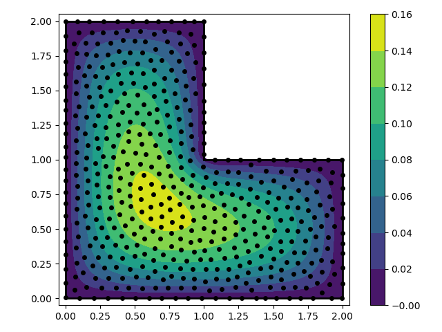
In this example we solve the Poisson equation over an L-shaped domain with
fixed boundary conditions. We use the RBF-FD method. The RBF-FD method is
preferable over the spectral RBF method because it is scalable and does not
require the user to specify a shape parameter (assuming that we use odd order
polyharmonic splines to generate the weights).
'''
import numpy as np
from scipy.sparse import coo_matrix
from scipy.sparse.linalg import spsolve
import matplotlib.pyplot as plt

from rbf.sputils import expand_rows
from rbf.pde.fd import weight_matrix
from rbf.pde.geometry import contains
from rbf.pde.nodes import poisson_disc_nodes

# Define the problem domain with line segments.
vert = np.array([[0.0, 0.0], [2.0, 0.0], [2.0, 1.0],
                 [1.0, 1.0], [1.0, 2.0], [0.0, 2.0]])
smp = np.array([[0, 1], [1, 2], [2, 3], [3, 4], [4, 5], [5, 0]])

spacing = 0.07 # approximate spacing between nodes

n = 25 # stencil size. Increase this will generally improve accuracy

phi = 'phs3' # radial basis function used to compute the weights. Odd
             # order polyharmonic splines (e.g., phs3) have always performed
             # well for me and they do not require the user to tune a shape
             # parameter. Use higher order polyharmonic splines for higher
             # order PDEs.

order = 2 # Order of the added polynomials. This should be at least as
          # large as the order of the PDE being solved (2 in this case). Larger
          # values may improve accuracy

# generate nodes
nodes, groups, _ = poisson_disc_nodes(spacing, (vert, smp)) 
N = nodes.shape[0]

# create the components for the "left hand side" matrix. 
A_interior = weight_matrix(
    x=nodes[groups['interior']], 
    p=nodes, 
    n=n,
    diffs=[[2, 0], [0, 2]],
    phi=phi, 
    order=order)
A_boundary = weight_matrix(
    x=nodes[groups['boundary:all']], 
    p=nodes, 
    n=1,
    diffs=[0, 0]) 
# Expand and add the components together
A  = expand_rows(A_interior, groups['interior'], N)
A += expand_rows(A_boundary, groups['boundary:all'], N)
                           
# create "right hand side" vector
d = np.zeros((N,))
d[groups['interior']] = -1.0
d[groups['boundary:all']] = 0.0

# find the solution at the nodes
u_soln = spsolve(A, d) 

# Create a grid for interpolating the solution
xg, yg = np.meshgrid(np.linspace(0.0, 2.02, 100), np.linspace(0.0, 2.02, 100))
points = np.array([xg.flatten(), yg.flatten()]).T                    

# We can use any method of scattered interpolation (e.g.,
# scipy.interpolate.LinearNDInterpolator). Here we repurpose the RBF-FD method
# to do the interpolation with a high order of accuracy
I = weight_matrix(
    x=points, 
    p=nodes, 
    n=n, 
    diffs=[0, 0],
    phi=phi,
    order=order)
u_itp = I.dot(u_soln)

# mask points outside of the domain
u_itp[~contains(points, vert, smp)] = np.nan 
ug = u_itp.reshape((100, 100)) # fold back into a grid

# make a contour plot of the solution
fig, ax = plt.subplots()
p = ax.contourf(xg, yg, ug, np.linspace(-1e-6, 0.16, 9), cmap='viridis')
ax.plot(nodes[:, 0], nodes[:, 1], 'ko', markersize=4)
for s in smp:
  ax.plot(vert[s, 0], vert[s, 1], 'k-', lw=2)

ax.set_aspect('equal')
ax.set_xlim(-0.05, 2.05)
ax.set_ylim(-0.05, 2.05)
fig.colorbar(p, ax=ax)
fig.tight_layout()
plt.savefig('../figures/fd.i.png')
plt.show()

''' 
In this example we solve the Poisson equation over an L-shaped domain with a
mix of free and fixed boundary conditions. We use the RBF-FD method and
demonstrate the use of ghost nodes along the free boundary.
'''
import numpy as np
from scipy.sparse.linalg import spsolve
from scipy.interpolate import LinearNDInterpolator
import matplotlib.pyplot as plt

from rbf.sputils import expand_rows
from rbf.pde.fd import weight_matrix
from rbf.pde.geometry import contains
from rbf.pde.nodes import poisson_disc_nodes


def series_solution(nodes, n=50):
    '''
    The analytical solution for this example
    '''
    x, y = nodes[:,0] - 1.0, nodes[:,1] - 1.0
    out = (1 - x**2)/2 
    for k in range(1, n+1, 2):
        out_k  = 16/np.pi**3
        out_k *= np.sin(k*np.pi*(1 + x)/2)/(k**3*np.sinh(k*np.pi))
        out_k *= (np.sinh(k*np.pi*(1 + y)/2) + 
                  np.sinh(k*np.pi*(1 - y)/2))
        out -= out_k

    return out

    
# Define the problem domain with line segments.
vert = np.array([[0.0, 0.0], [2.0, 0.0], [2.0, 1.0],
                 [1.0, 1.0], [1.0, 2.0], [0.0, 2.0]])
smp = np.array([[0, 1], [1, 2], [4, 5], [5, 0], [2, 3], [3, 4]])
# define which simplices make up the free and fixed boundary conditions
boundary_groups = {'fixed': [0, 1, 2, 3],
                   'free': [4, 5]}

spacing = 0.1  # The approximate spacing between nodes

n = 25 # stencil size. Increasing this will generally improve accuracy

phi = 'phs5' # radial basis function used to compute the weights. Odd
             # order polyharmonic splines (e.g., phs3) have always performed
             # well for me and they do not require the user to tune a shape
             # parameter. Use higher order polyharmonic splines for higher
             # order PDEs.

order = 4 # Order of the added polynomials. This should be at least as
          # large as the order of the PDE being solved (2 in this case). Larger
          # values may improve accuracy

# generate nodes
nodes, groups, normals = poisson_disc_nodes(
    spacing, 
    (vert, smp), 
    boundary_groups=boundary_groups,
    boundary_groups_with_ghosts=['free'])
N = nodes.shape[0] 

# create the components for the "left hand side" matrix.  

# create the components to evaluate the PDE at the interior and boundary
A_interior = weight_matrix(
    x=nodes[groups['interior']], 
    p=nodes, 
    n=n,
    diffs=[[2, 0], [0, 2]], 
    phi=phi, 
    order=order)

A_ghost = weight_matrix(
    x=nodes[groups['boundary:free']], 
    p=nodes, 
    n=n,
    diffs=[[2, 0], [0, 2]],
    phi=phi, 
    order=order)

# create the component for the fixed boundary conditions. This is essentially
# an identity operation and so we only need a stencil size of 1
A_fixed = weight_matrix(
    x=nodes[groups['boundary:fixed']], 
    p=nodes, 
    n=1,
    diffs=[0, 0]) 

# create the component for the free boundary conditions. This dots the
# derivative with respect to x and y with the x and y components of normal
# vectors on the free surface (i.e., n_x * du/dx + n_y * du/dy)
A_free = weight_matrix(
    x=nodes[groups['boundary:free']], 
    p=nodes, 
    n=n,
    diffs=[[1, 0], [0, 1]],
    coeffs=[normals[groups['boundary:free'], 0],
            normals[groups['boundary:free'], 1]],
    phi=phi, 
    order=order)
                           
# Add the components to the corresponding rows of `A`
A  = expand_rows(A_interior, groups['interior'], N)
A += expand_rows(A_ghost, groups['ghosts:free'], N)
A += expand_rows(A_fixed, groups['boundary:fixed'], N)
A += expand_rows(A_free, groups['boundary:free'], N)
                           
# create "right hand side" vector
d = np.zeros((N,))
d[groups['interior']] = -1.0
d[groups['ghosts:free']] = -1.0
d[groups['boundary:fixed']] = 0.0
d[groups['boundary:free']] = 0.0

# find the solution and error at the nodes
u_soln = spsolve(A, d) 
error = np.abs(u_soln - series_solution(nodes))

## PLOT THE NUMERICAL SOLUTION AND ITS ERROR
fig, axs = plt.subplots(2, figsize=(6, 8))
# interpolate the solution on a grid
xg, yg = np.meshgrid(np.linspace(-0.05, 2.05, 400), 
                     np.linspace(-0.05, 2.05, 400))
points = np.array([xg.flatten(), yg.flatten()]).T  
u_itp = LinearNDInterpolator(nodes, u_soln)(points)
# mask points outside of the domain
u_itp[~contains(points, vert, smp)] = np.nan 
ug = u_itp.reshape((400, 400)) # fold back into a grid
# make a contour plot of the solution
p = axs[0].contourf(xg, yg, ug, np.linspace(-1e-6, 0.3, 9), cmap='viridis')
fig.colorbar(p, ax=axs[0])
# plot the domain
for s in smp:
  axs[0].plot(vert[s, 0], vert[s, 1], 'k-', lw=2)

# show the locations of the nodes
for i, (k, v)  in enumerate(groups.items()):
    axs[0].plot(nodes[v, 0], nodes[v, 1], 'C%so' % i, markersize=4, label=k)

axs[0].set_title('RBF-FD solution')
axs[0].set_aspect('equal')
axs[0].legend()

# plot the error at the location of the non-ghost nodes 
idx_no_ghosts = np.hstack((groups['interior'], 
                           groups['boundary:free'],
                           groups['boundary:fixed']))
p = axs[1].scatter(nodes[idx_no_ghosts, 0], 
                   nodes[idx_no_ghosts, 1], 
                   s=20, c=error[idx_no_ghosts])
fig.colorbar(p, ax=axs[1])
# make the background black so its easier to see the colors
axs[1].set_facecolor('k')
axs[1].set_title('Error')
axs[1].set_aspect('equal')

fig.tight_layout()

plt.savefig('../figures/fd.j.png')
plt.show()

''' 
This script demonstrates using the RBF-FD method to calculate static
deformation of a two-dimensional elastic material subject to a uniform body
force such as gravity. The elastic material has a fixed boundary condition on
one side and the remaining sides have a free surface boundary condition.  This
script also demonstrates using ghost nodes which, for all intents and purposes,
are necessary when dealing with Neumann boundary conditions.
'''
import logging

import numpy as np
import scipy.sparse as sp
import matplotlib.pyplot as plt
from matplotlib.colors import LogNorm

from rbf.sputils import expand_rows
from rbf.linalg import GMRESSolver
from rbf.pde.fd import weight_matrix
from rbf.pde.nodes import poisson_disc_nodes

logging.basicConfig(level=logging.DEBUG)

## User defined parameters
#####################################################################
# define the vertices of the problem domain. Note that the first simplex will
# be fixed, and the others will be free
vert = np.array([[0.0, 0.0], [0.0, 1.0], [2.0, 1.0], [2.0, 0.0]])
smp = np.array([[0, 1], [1, 2], [2, 3], [3, 0]])
# The node spacing
dx = 0.05
# size of RBF-FD stencils
n = 30
# lame parameters
lamb = 1.0
mu = 1.0
# z component of body for
body_force = 1.0

## Build and solve for displacements and strain
#####################################################################
# generate nodes. The nodes are assigned groups based on which simplex they lay
# on
boundary_groups = {'fixed':[0], 'free':[1, 2, 3]}
nodes, groups, normals = poisson_disc_nodes(
    dx, 
    (vert, smp),
    boundary_groups=boundary_groups,
    boundary_groups_with_ghosts=['free'])
N = nodes.shape[0]
# `nodes` : (N, 2) float array
# `groups` : dictionary containing index sets. It has the keys
#            "interior", "boundary:free", "boundary:fixed",
#            "ghosts:free".
# `normals : (N, 2) float array

## Enforce the PDE on interior nodes AND the free surface nodes 
# x component of force resulting from displacement in the x direction.
coeffs_xx = [lamb+2*mu, mu]
diffs_xx = [(2, 0), (0, 2)]
# x component of force resulting from displacement in the y direction.
coeffs_xy = [lamb, mu]
diffs_xy = [(1, 1), (1, 1)]
# y component of force resulting from displacement in the x direction.
coeffs_yx = [mu, lamb]
diffs_yx = [(1, 1), (1, 1)]
# y component of force resulting from displacement in the y direction.
coeffs_yy = [lamb+2*mu, mu]
diffs_yy =  [(0, 2), (2, 0)]
# make the differentiation matrices that enforce the PDE on the interior nodes.
D_xx = weight_matrix(nodes[groups['interior']], nodes, n, diffs_xx, coeffs=coeffs_xx)
D_xy = weight_matrix(nodes[groups['interior']], nodes, n, diffs_xy, coeffs=coeffs_xy)
D_yx = weight_matrix(nodes[groups['interior']], nodes, n, diffs_yx, coeffs=coeffs_yx)
D_yy = weight_matrix(nodes[groups['interior']], nodes, n, diffs_yy, coeffs=coeffs_yy)
G_xx = expand_rows(D_xx, groups['interior'], N)
G_xy = expand_rows(D_xy, groups['interior'], N)
G_yx = expand_rows(D_yx, groups['interior'], N)
G_yy = expand_rows(D_yy, groups['interior'], N)

# use the ghost nodes to enforce the PDE on the boundary
D_xx = weight_matrix(nodes[groups['boundary:free']], nodes, n, diffs_xx, coeffs=coeffs_xx)
D_xy = weight_matrix(nodes[groups['boundary:free']], nodes, n, diffs_xy, coeffs=coeffs_xy)
D_yx = weight_matrix(nodes[groups['boundary:free']], nodes, n, diffs_yx, coeffs=coeffs_yx)
D_yy = weight_matrix(nodes[groups['boundary:free']], nodes, n, diffs_yy, coeffs=coeffs_yy)
G_xx += expand_rows(D_xx, groups['ghosts:free'], N)
G_xy += expand_rows(D_xy, groups['ghosts:free'], N)
G_yx += expand_rows(D_yx, groups['ghosts:free'], N)
G_yy += expand_rows(D_yy, groups['ghosts:free'], N)

## Enforce fixed boundary conditions
# Enforce that x and y are as specified with the fixed boundary condition.
# These matrices turn out to be identity matrices, but I include this
# computation for consistency with the rest of the code. feel free to comment
# out the next couple lines and replace it with an appropriately sized sparse
# identity matrix.
coeffs_xx = [1.0]
diffs_xx = [(0, 0)]
coeffs_yy = [1.0]
diffs_yy = [(0, 0)]

dD_fix_xx = weight_matrix(nodes[groups['boundary:fixed']], nodes, n, diffs_xx, coeffs=coeffs_xx)
dD_fix_yy = weight_matrix(nodes[groups['boundary:fixed']], nodes, n, diffs_yy, coeffs=coeffs_yy)
G_xx += expand_rows(dD_fix_xx, groups['boundary:fixed'], N)
G_yy += expand_rows(dD_fix_yy, groups['boundary:fixed'], N)

## Enforce free surface boundary conditions
# x component of traction force resulting from x displacement 
coeffs_xx = [normals[groups['boundary:free']][:, 0]*(lamb+2*mu), 
             normals[groups['boundary:free']][:, 1]*mu]
diffs_xx = [(1, 0), (0, 1)]
# x component of traction force resulting from y displacement
coeffs_xy = [normals[groups['boundary:free']][:, 0]*lamb, 
             normals[groups['boundary:free']][:, 1]*mu]
diffs_xy = [(0, 1), (1, 0)]
# y component of traction force resulting from x displacement
coeffs_yx = [normals[groups['boundary:free']][:, 0]*mu, 
             normals[groups['boundary:free']][:, 1]*lamb]
diffs_yx = [(0, 1), (1, 0)]
# y component of force resulting from displacement in the y direction
coeffs_yy = [normals[groups['boundary:free']][:, 1]*(lamb+2*mu), 
             normals[groups['boundary:free']][:, 0]*mu]
diffs_yy =  [(0, 1), (1, 0)]
# make the differentiation matrices that enforce the free surface boundary 
# conditions.
dD_free_xx = weight_matrix(nodes[groups['boundary:free']], nodes, n, diffs_xx, coeffs=coeffs_xx)
dD_free_xy = weight_matrix(nodes[groups['boundary:free']], nodes, n, diffs_xy, coeffs=coeffs_xy)
dD_free_yx = weight_matrix(nodes[groups['boundary:free']], nodes, n, diffs_yx, coeffs=coeffs_yx)
dD_free_yy = weight_matrix(nodes[groups['boundary:free']], nodes, n, diffs_yy, coeffs=coeffs_yy)

G_xx += expand_rows(dD_free_xx, groups['boundary:free'], N)
G_xy += expand_rows(dD_free_xy, groups['boundary:free'], N)
G_yx += expand_rows(dD_free_yx, groups['boundary:free'], N)
G_yy += expand_rows(dD_free_yy, groups['boundary:free'], N)

# stack the components together to form the left-hand-side matrix
G_x = sp.hstack((G_xx, G_xy))
G_y = sp.hstack((G_yx, G_yy))
G = sp.vstack((G_x, G_y))

# form the right-hand-side vector
d_x = np.zeros((N,))
d_y = np.zeros((N,))

d_x[groups['interior']] = 0.0
d_x[groups['ghosts:free']] = 0.0
d_x[groups['boundary:free']] = 0.0
d_x[groups['boundary:fixed']] = 0.0

d_y[groups['interior']] = body_force
d_y[groups['ghosts:free']] = body_force
d_y[groups['boundary:free']] = 0.0
d_y[groups['boundary:fixed']] = 0.0

d = np.hstack((d_x, d_y))

# solve the system!
u = GMRESSolver(G).solve(d)

# reshape the solution
u = np.reshape(u, (2, -1))
u_x, u_y = u

## Calculate strain on a fine grid from displacements
x, y = np.meshgrid(np.linspace(0.0, 2.0, 100), np.linspace(0.0, 1.0, 50))
points = np.array([x.flatten(), y.flatten()]).T

D_x = weight_matrix(points, nodes, n, (1, 0))
D_y = weight_matrix(points, nodes, n, (0, 1))
e_xx = D_x.dot(u_x)
e_yy = D_y.dot(u_y)
e_xy = 0.5*(D_y.dot(u_x) + D_x.dot(u_y))
# calculate second strain invariant
I2 = np.sqrt(e_xx**2 + e_yy**2 + 2*e_xy**2)

## Plot the results
#####################################################################
idx_no_ghosts = np.hstack((groups['interior'],
                           groups['boundary:free'],
                           groups['boundary:fixed']))
                          
nodes = nodes[idx_no_ghosts]
u_x = u_x[idx_no_ghosts]
u_y = u_y[idx_no_ghosts]

fig, ax = plt.subplots(figsize=(7, 3.5))
# plot the fixed boundary
ax.plot(vert[smp[0], 0], vert[smp[0], 1], 'r-', lw=2, label='fixed', zorder=1)
# plot the free boundary
ax.plot(vert[smp[1], 0], vert[smp[1], 1], 'r--', lw=2, label='free', zorder=1)
for s in smp[2:]:
  ax.plot(vert[s, 0], vert[s, 1], 'r--', lw=2, zorder=1)

# plot the second strain invariant
p = ax.tripcolor(points[:, 0], points[:, 1], I2,
                 norm=LogNorm(vmin=0.1, vmax=3.2),
                 cmap='viridis', zorder=0)
# plot the displacement vectors
ax.quiver(nodes[:, 0], nodes[:, 1], u_x, u_y, zorder=2)
ax.set_xlim((-0.1, 2.1))
ax.set_ylim((-0.25, 1.1))
ax.set_aspect('equal')
ax.legend(loc=3, frameon=False, fontsize=12, ncol=2)
cbar = fig.colorbar(p)
cbar.set_label('second strain invariant')
fig.tight_layout()
plt.savefig('../figures/fd.b.png')
plt.show() 

'''
This script solves the 2-D wave equation on an L-shaped domain with free
boundary conditions. This also illustrates how to implement hyperviscosity to
stabilize the time stepping.
'''
import logging

import numpy as np
import matplotlib.pyplot as plt
from matplotlib.animation import FuncAnimation

from scipy.sparse.linalg import splu, LinearOperator, eigs
from scipy.integrate import solve_ivp

from rbf.sputils import expand_rows, expand_cols
from rbf.pde.fd import weight_matrix
from rbf.pde.nodes import poisson_disc_nodes
from rbf.pde.geometry import contains

logging.basicConfig(level=logging.DEBUG)

# define the problem domain
vert = np.array([[0.0, 0.0],
                 [2.0, 0.0],
                 [2.0, 1.0],
                 [1.0, 1.0],
                 [1.0, 2.0],
                 [0.0, 2.0]])
smp = np.array([[0, 1],
                [1, 2],
                [2, 3],
                [3, 4],
                [4, 5],
                [5, 0]])
# the times where we will evaluate the solution (these are not the time steps)
times = np.linspace(0.0, 4.0, 41)
# the spacing between nodes
spacing = 0.05
# the wave speed
rho = 1.0 
# the hyperviscosity factor
nu = 1e-6
# whether to plot the eigenvalues for the state differentiation matrix. All the
# eigenvalues must have a negative real component for the time stepping to be
# stable
plot_eigs = True
# number of nodes used for each RBF-FD stencil
stencil_size = 50
# the polynomial order for generating the RBF-FD weights
order = 4
# the RBF used for generating the RBF-FD weights
phi = 'phs5'

# generate the nodes
nodes, groups, normals = poisson_disc_nodes(
    spacing,
    (vert, smp),
    boundary_groups={'all':range(len(smp))},
    boundary_groups_with_ghosts=['all'])
n = nodes.shape[0]

# We will solve the wave equation by numerically integrating the state vector
# `z`. The state vector is a concatenation of `u` and `v`. `u` is a (n,) array
# consisting of:
#
#     - the displacements at the interior at `u[groups['interior']]`
#     - the displacements at the boundary at `u[groups['boundary:all']]`
#     - the free boundary conditions at `u[groups['ghosts:all']]`
#
# `v` is a (n,) array and it is the time derivative of `u`

# create a new node group for convenience
groups['interior+boundary:all'] = np.hstack((groups['interior'],
                                             groups['boundary:all']))

# create the initial displacements at the interior and boundary, the velocities
# are zero
r = np.sqrt((nodes[groups['interior+boundary:all'], 0] - 0.5)**2 +
            (nodes[groups['interior+boundary:all'], 1] - 0.5)**2)

u_init = np.zeros((n,))
u_init[groups['interior+boundary:all']] = 1.0/(1 + (r/0.1)**4)
v_init = np.zeros((n,))
z_init = np.hstack((u_init, v_init))

# construct a matrix that maps the displacements at `nodes` to `u`
B_disp = weight_matrix(
    x=nodes[groups['interior+boundary:all']],
    p=nodes,
    n=1,
    diffs=(0, 0))
B_free = weight_matrix(
    x=nodes[groups['boundary:all']],
    p=nodes,
    n=stencil_size,
    diffs=[(1, 0), (0, 1)],
    coeffs=[normals[groups['boundary:all'], 0],
            normals[groups['boundary:all'], 1]],
    phi=phi,
    order=order)
B  = expand_rows(B_disp, groups['interior+boundary:all'], n)
B += expand_rows(B_free, groups['ghosts:all'], n)
B = B.tocsc()
Bsolver = splu(B)

# construct a matrix that maps the displacements at `nodes` to the acceleration
# of `u` due to body forces.
D = rho*weight_matrix(
    x=nodes[groups['interior+boundary:all']],
    p=nodes,
    n=stencil_size,
    diffs=[(2, 0), (0, 2)],
    phi=phi,
    order=order)
D = expand_rows(D, groups['interior+boundary:all'], n)
D = D.tocsc()

# construct a matrix that maps `v` to the acceleration of `u` due to
# hyperviscosity.
H = -nu*weight_matrix(
    x=nodes[groups['interior+boundary:all']],
    p=nodes[groups['interior+boundary:all']],
    n=stencil_size,
    diffs=[(4, 0), (2, 2), (0, 4)],
    coeffs=[1.0, 2.0, 1.0],
    phi='phs5',
    order=4)
H = expand_rows(H, groups['interior+boundary:all'], n)
H = expand_cols(H, groups['interior+boundary:all'], n)
H = H.tocsc()

# create a function used for time stepping. this returns the time derivative of
# the state vector
def state_derivative(t, z):
    u, v = z.reshape((2, -1))
    return np.hstack([v, D.dot(Bsolver.solve(u)) + H.dot(v)])

if plot_eigs:
    L = LinearOperator((2*n, 2*n), matvec=lambda x:state_derivative(0.0, x))
    print('computing eigenvectors ...')
    vals = eigs(L, 2*n - 2, return_eigenvectors=False)
    print('done')
    print('min real: %s' % np.min(vals.real))
    print('max real: %s' % np.max(vals.real))
    print('min imaginary: %s' % np.min(vals.imag))
    print('max imaginary: %s' % np.max(vals.imag))
    fig, ax = plt.subplots()
    ax.plot(vals.real, vals.imag, 'ko')
    ax.set_title('eigenvalues of the state differentiation matrix')
    ax.set_xlabel('real')
    ax.set_ylabel('imaginary')
    ax.grid(ls=':')
    plt.savefig('../figures/fd.d.1.png')

print('performing time integration ...')
soln = solve_ivp(
    fun=state_derivative,
    t_span=[times[0], times[-1]],
    y0=z_init,
    method='RK45',
    t_eval=times)
print('done')


## PLOTTING
# create the interpolation points
xgrid, ygrid = np.meshgrid(np.linspace(0.0, 2.01, 100),
                           np.linspace(0.0, 2.01, 100))
xy = np.array([xgrid.flatten(), ygrid.flatten()]).T

# create an interpolation matrix that maps `u` to the displacements at `xy`
I = weight_matrix(
    x=xy, 
    p=nodes[groups['interior+boundary:all']], 
    n=stencil_size, 
    diffs=(0, 0), 
    phi=phi,
    order=order)
I = expand_cols(I, groups['interior+boundary:all'], n)

# create a mask for points in `xy` that are outside of the domain
is_outside = ~contains(xy, vert, smp)

fig = plt.figure()

# create the update function for the animation. this plots the solution at time
# `time[index]`
def update(index):
    fig.clear()
    ax = fig.add_subplot(111)

    u, v = soln.y[:, index].reshape((2, -1))
    u_xy = I.dot(u)
    u_xy[is_outside] = np.nan 
    u_xy = u_xy.reshape((100, 100))

    for s in smp:
        ax.plot(vert[s, 0], vert[s, 1], 'k-')

    p = ax.contourf(
        xgrid, ygrid, u_xy, 
        np.linspace(-0.4, 0.4, 21), 
        cmap='seismic',
        extend='both')

    ax.scatter(nodes[:, 0], nodes[:, 1], c='k', s=2)
    ax.set_title('time: %.2f' % times[index])

    ax.set_xlim(-0.05, 2.05)     
    ax.set_ylim(-0.05, 2.05)     
    ax.grid(ls=':', color='k')   
    ax.set_aspect('equal')
    fig.colorbar(p)
    fig.tight_layout()

    return

ani = FuncAnimation(
    fig=fig, 
    func=update, 
    frames=range(len(times)), 
    repeat=True,
    blit=False)
    
ani.save('../figures/fd.d.2.gif', writer='imagemagick', fps=3)
plt.show()

'''
This script demonstrates using RBF-FD to solve Poisson's equation with mixed
boundary conditions on a domain with a hole inside of it.
'''
import logging

import matplotlib.pyplot as plt
import numpy as np
import scipy.sparse as sp

from rbf.pde.nodes import poisson_disc_nodes
from rbf.pde.fd import weight_matrix
from rbf.pde.geometry import contains
from rbf.interpolate import KNearestRBFInterpolant

logging.basicConfig(level=logging.DEBUG)

node_spacing = 0.25
radial_basis_function = 'phs3' # 3rd order polyharmonic spline
polynomial_order = 2
stencil_size = 30 

vertices = np.array(
    [[-2.    ,  2.    ], [ 2.    ,  2.    ], [ 2.    , -2.    ],
     [-2.    , -2.    ], [ 1.    ,  0.    ], [ 0.9239,  0.3827],
     [ 0.7071,  0.7071], [ 0.3827,  0.9239], [ 0.    ,  1.    ],
     [-0.3827,  0.9239], [-0.7071,  0.7071], [-0.9239,  0.3827],
     [-1.    ,  0.    ], [-0.9239, -0.3827], [-0.7071, -0.7071],
     [-0.3827, -0.9239], [-0.    , -1.    ], [ 0.3827, -0.9239],
     [ 0.7071, -0.7071], [ 0.9239, -0.3827]]
    )

simplices = np.array(
    [[0 , 1 ], [1 , 2 ], [2 , 3 ], [3 , 0 ], [4 , 5 ], [5 , 6 ], [6 , 7 ],
     [7 , 8 ], [8 , 9 ], [9 , 10], [10, 11], [11, 12], [12, 13], [13, 14],
     [14, 15], [15, 16], [16, 17], [17, 18], [18, 19], [19,  4]]
    )     

boundary_groups = {
    'box': [0, 1, 2, 3],
    'circle': [4, 5, 6, 7, 8, 9, 10, 11, 12, 13, 14, 15, 16, 17, 18, 19]
    }
    
# Generate the nodes. `groups` identifies which group each node belongs to.
# `normals` contains the normal vectors corresponding to each node (nan if the
# node is not on a boundary). We are giving the circle boundary nodes ghost
# nodes to improve the accuracy of the free boundary constraint.
nodes, groups, normals = poisson_disc_nodes(
    node_spacing,
    (vertices, simplices),
    boundary_groups=boundary_groups,
    boundary_groups_with_ghosts=['circle']
    )

# Create the LHS and RHS enforcing that the Lapacian is -5 at the interior
# nodes
A_interior = weight_matrix(
    nodes[groups['interior']],
    nodes,
    stencil_size,
    [[2, 0], [0, 2]],
    phi=radial_basis_function,
    order=polynomial_order
    )

b_interior = np.full(len(groups['interior']), -5.0)

# Enforce that the solution is x at the box boundary nodes.
A_boundary_box = weight_matrix(
    nodes[groups['boundary:box']],
    nodes,
    stencil_size,
    [0, 0],
    phi=radial_basis_function,
    order=polynomial_order
    )

b_boundary_box = nodes[groups['boundary:box'], 0]

# Enforce a free boundary at the circle boundary nodes.
A_boundary_circle = weight_matrix(
    nodes[groups['boundary:circle']],
    nodes,
    stencil_size,
    [[1, 0], [0, 1]],
    coeffs=[
        normals[groups['boundary:circle'], 0],
        normals[groups['boundary:circle'], 1]
        ],
    phi=radial_basis_function,
    order=polynomial_order
    )

b_boundary_circle = np.zeros(len(groups['boundary:circle']))

# Use the extra degrees of freedom from the ghost nodes to enforce that the
# Laplacian is -5 at the circle boundary nodes.
A_ghosts_circle = weight_matrix(
    nodes[groups['boundary:circle']],
    nodes,
    stencil_size,
    [[2, 0], [0, 2]],
    phi=radial_basis_function,
    order=polynomial_order
    )

b_ghosts_circle = np.full(len(groups['boundary:circle']), -5.0)

# Combine the LHS and RHS components and solve
A = sp.vstack(
    (A_interior, A_boundary_box, A_boundary_circle, A_ghosts_circle)
    ).tocsc()

b = np.hstack(
    (b_interior, b_boundary_box, b_boundary_circle, b_ghosts_circle)
    )

soln = sp.linalg.spsolve(A, b)

# The rest is just plotting...
fig, ax = plt.subplots()
for smp in simplices:
    ax.plot(vertices[smp, 0], vertices[smp, 1], 'k-')

for name, idx in groups.items():
    ax.plot(nodes[idx, 0], nodes[idx, 1], '.', label=name)

points_grid = np.mgrid[
    nodes[:, 0].min():nodes[:, 0].max():200j,
    nodes[:, 1].min():nodes[:, 1].max():200j,
    ]

points_flat = points_grid.reshape(2, -1).T
soln_interp_flat = KNearestRBFInterpolant(
    nodes, soln,
    phi=radial_basis_function,
    k=stencil_size,
    order=polynomial_order
    )(points_flat)
    
soln_interp_flat[~contains(points_flat, vertices, simplices)] = np.nan
soln_interp_grid = soln_interp_flat.reshape(points_grid.shape[1:])
p = ax.contourf(*points_grid, soln_interp_grid, cmap='jet')
fig.colorbar(p)
ax.legend(loc=2)
ax.grid(ls=':')
ax.set_xlim(-2.5, 2.5)
ax.set_ylim(-2.5, 2.5)
ax.set_aspect('equal')
ax.set_title('Interpolated solution')
fig.tight_layout()
plt.savefig('../figures/fd.m.png')
plt.show()

'''
This script demonstrates using RBF-FD to solve the heat equation with spatially
variable conductivity, k(x, y). Namely,

    u_t = k_x*u_x + k*u_xx + k_y*u_y + k*u_yy

'''
import logging

import matplotlib.pyplot as plt
from matplotlib.animation import FuncAnimation
import numpy as np
from scipy.sparse.linalg import splu
from scipy.integrate import solve_ivp

from rbf.pde.nodes import poisson_disc_nodes
from rbf.pde.fd import weight_matrix
from rbf.pde.geometry import contains
from rbf.sputils import expand_rows, expand_cols

logging.basicConfig(level=logging.DEBUG)

node_spacing = 0.1
radial_basis_function = 'phs3' # 3rd order polyharmonic spline
polynomial_order = 2
stencil_size = 30
time_evaluations = np.linspace(0, 1, 41)

vertices = np.array(
    [[-2.    ,  2.    ], [ 2.    ,  2.    ], [ 2.    , -2.    ],
     [-2.    , -2.    ], [ 1.    ,  0.    ], [ 0.9239,  0.3827],
     [ 0.7071,  0.7071], [ 0.3827,  0.9239], [ 0.    ,  1.    ],
     [-0.3827,  0.9239], [-0.7071,  0.7071], [-0.9239,  0.3827],
     [-1.    ,  0.    ], [-0.9239, -0.3827], [-0.7071, -0.7071],
     [-0.3827, -0.9239], [-0.    , -1.    ], [ 0.3827, -0.9239],
     [ 0.7071, -0.7071], [ 0.9239, -0.3827]]
    )

simplices = np.array(
    [[0 , 1 ], [1 , 2 ], [2 , 3 ], [3 , 0 ], [4 , 5 ], [5 , 6 ], [6 , 7 ],
     [7 , 8 ], [8 , 9 ], [9 , 10], [10, 11], [11, 12], [12, 13], [13, 14],
     [14, 15], [15, 16], [16, 17], [17, 18], [18, 19], [19,  4]]
    )

boundary_groups = {
    'fixed': [1, 3],
    'free': [0, 2, 4, 5, 6, 7, 8, 9, 10, 11, 12, 13, 14, 15, 16, 17, 18, 19]
    }

def conductivity(x):
    out = 1 + 3*(1 / (1 + np.exp(-5*x[:, 1])))
    return out

def conductivity_xdiff(x):
    # finite difference x derivative of conductivity
    delta = 1e-3
    out = (conductivity(x + [delta, 0.0]) - conductivity(x))/delta
    return out

def conductivity_ydiff(x):
    # finite difference y derivative of conductivity
    delta = 1e-3
    out = (conductivity(x + [0.0, delta]) - conductivity(x))/delta
    return out

# Generate the nodes. `groups` identifies which group each node belongs to.
# `normals` contains the normal vectors corresponding to each node (nan if the
# node is not on a boundary). We are giving the free boundary nodes ghost
# nodes to improve the accuracy of the free boundary constraint.
nodes, grp, normals = poisson_disc_nodes(
    node_spacing,
    (vertices, simplices),
    boundary_groups=boundary_groups,
    boundary_groups_with_ghosts=['free']
    )

# We will solve the heat equation by numerically integrating the state vector
# `z`. The state vector consists of:
#   - The temperature of the interior nodes at z[grp['interior']]
#   - The temperature of the fixed boundary at z[grp['boundary:fixed']]
#   - The temperature of the free boundary at z[grp['boundary:free']]
#   - The boundary condition at the free boundary at z[grp['ghosts:free']]
#
z_init = np.zeros(nodes.shape[0])
z_init[grp['boundary:fixed']] = nodes[grp['boundary:fixed'], 0]

# Create a matrix that maps the temperature at `nodes` to the state vector.
# Then create a solver for it, so we can map the state vector to the
# temperature at all nodes.

# `idx` are the indices for all nodes except the ghost nodes. The mapping to
# the state vector is just an identity mapping so we only need a stencil size
# of 1.
idx = np.hstack((grp['interior'], grp['boundary:fixed'], grp['boundary:free']))
B_temp = weight_matrix(
    x=nodes[idx],
    p=nodes,
    n=1,
    diffs=[0, 0]
    )
B_free = weight_matrix(
    x=nodes[grp['boundary:free']],
    p=nodes,
    n=stencil_size,
    diffs=[[1, 0], [0, 1]],
    coeffs=[
        normals[grp['boundary:free'], 0],
        normals[grp['boundary:free'], 1]
        ],
    phi=radial_basis_function,
    order=polynomial_order
    )

B = expand_rows(B_temp, idx, nodes.shape[0])
B += expand_rows(B_free, grp['ghosts:free'], nodes.shape[0])
B = B.tocsc()
Bsolver = splu(B)

# construct a matrix that maps the temperature at `nodes` to the time
# derivative of the state vector

# `idx` are the indices of the state vector with a non-zero time derivative
# (i.e., the elements of the state vector that are not enforcing the boundary
# conditions).
idx = np.hstack((grp['interior'], grp['boundary:free']))
A = weight_matrix(
    x=nodes[idx],
    p=nodes,
    n=stencil_size,
    diffs=[[1, 0], [2, 0], [0, 1], [0, 2]],
    coeffs=[
        conductivity_xdiff(nodes[idx]),
        conductivity(nodes[idx]),
        conductivity_ydiff(nodes[idx]),
        conductivity(nodes[idx])
        ],
    phi=radial_basis_function,
    order=polynomial_order
    )
A = expand_rows(A, idx, nodes.shape[0])
A = A.tocsc()

def state_derivative(t, z):
    return A.dot(Bsolver.solve(z))

soln = solve_ivp(
    fun=state_derivative,
    t_span=[time_evaluations[0], time_evaluations[-1]],
    y0=z_init,
    method='RK45',
    t_eval=time_evaluations
    )

## PLOTTING
# create the interpolation points
xy_grid = np.mgrid[-2.01:2.01:200j, -2.01:2.01:200j]
xy = xy_grid.reshape(2, -1).T

# create an interpolation matrix that maps the state vector to the temperature
# at `xy`. `idx` consists of indices of the state vector that are temperatures.
idx = np.hstack((grp['interior'], grp['boundary:fixed'], grp['boundary:free']))
I = weight_matrix(
    x=xy,
    p=nodes[idx],
    n=stencil_size,
    diffs=[0, 0],
    phi=radial_basis_function,
    order=polynomial_order
    )
I = expand_cols(I, idx, nodes.shape[0])

# create a mask for points in `xy` that are outside of the domain
is_outside = ~contains(xy, vertices, simplices)

fig1, ax1  = plt.subplots()
k = conductivity(xy)
k[is_outside] = np.nan
k = k.reshape(200, 200)
p = ax1.contourf(*xy_grid, k, np.linspace(1, 4, 11), cmap='viridis')

for smp in simplices:
    ax1.plot(vertices[smp, 0], vertices[smp, 1], 'k-', zorder=1)

for i, (k, v) in enumerate(grp.items()):
    ax1.scatter(nodes[v, 0], nodes[v, 1], s=10, c='C%d' % i, label=k, zorder=2)

ax1.set_aspect('equal')
ax1.set_xlim(-2.2, 2.2)
ax1.set_ylim(-2.2, 2.2)
ax1.grid(ls=':', color='k')
ax1.legend()
cbar = fig1.colorbar(p)
cbar.set_label('heat conductivity')
fig1.tight_layout()
plt.savefig('../figures/fd.n.1.png')

fig2 = plt.figure()
# create the update function for the animation. this plots the solution at time
# `time[index]`
def update(index):
    fig2.clear()
    ax2 = fig2.add_subplot(111)

    z = soln.y[:, index]
    temp = I.dot(z)
    temp[is_outside] = np.nan
    temp = temp.reshape((200, 200))

    for s in simplices:
        ax2.plot(vertices[s, 0], vertices[s, 1], 'k-')

    p = ax2.contourf(
        *xy_grid,
        temp,
        np.linspace(-2.0, 2.0, 10),
        cmap='viridis',
        extend='both'
        )

    ax2.scatter(nodes[:, 0], nodes[:, 1], c='k', s=2)
    ax2.set_title('temperature at time: %.2f' % time_evaluations[index])

    ax2.set_xlim(-2.1, 2.1)
    ax2.set_ylim(-2.1, 2.1)
    ax2.grid(ls=':', color='k')
    ax2.set_aspect('equal')
    fig2.colorbar(p)
    fig2.tight_layout()

ani = FuncAnimation(
    fig=fig2,
    func=update,
    frames=range(len(time_evaluations)),
    repeat=True,
    blit=False
    )

ani.save('../figures/fd.n.2.gif', writer='imagemagick', fps=3)
plt.show()