interpolate
This module provides a class for RBF interpolation, RBFInterpolant.
RBF Interpolation
An RBF interpolant fits scalar valued observations \(\mathbf{d}=[d_1,...,d_N]^T\) made at the distinct scattered locations \(y_1,...,y_N\). The RBF interpolant is parameterized as
where \(\phi\) is an RBF and \(p_1(x),...,p_M(x)\) are monomials that span the space of polynomials with a specified degree. The coefficients \(\mathbf{a}=[a_1,...,a_N]^T\) and \(\mathbf{b}=[b_1,...,b_M]^T\) are the solutions to the linear equations
and
where \(\mathbf{K}\) is a matrix with components \(K_{ij} = \phi(||y_i - y_j||_2)\), \(\mathbf{P}\) is a matrix with components \(P_{ij}=p_j(y_i)\), and \(\sigma\) is a smoothing parameter that controls how well we want to fit the observations. The observations are fit exactly when \(\sigma\) is zero.
If the chosen RBF is positive definite (see rbf.basis) and \(\mathbf{P}\) has full column rank, the solution for \(\mathbf{a}\) and \(\mathbf{b}\) is unique. If the chosen RBF is conditionally positive definite of order q and \(\mathbf{P}\) has full column rank, the solution is unique provided that the degree of the monomial terms is at least q-1 (see Chapter 7 of [1] or [2]).
References
[1] Fasshauer, G., 2007. Meshfree Approximation Methods with Matlab. World Scientific Publishing Co.
[2] http://amadeus.math.iit.edu/~fass/603_ch3.pdf
[3] Wahba, G., 1990. Spline Models for Observational Data. SIAM.
[4] http://pages.stat.wisc.edu/~wahba/stat860public/lect/lect8/lect8.pdf
- class rbf.interpolate.RBFInterpolant(y, d, sigma=0.0, phi='phs3', eps=1.0, order=None, neighbors=None, check_cond=True)
Radial basis function interpolant for scattered data.
- Parameters:
y ((N, D) float array) – Observation points.
d ((N, ...) float or complex array) – Observed values at y.
sigma (float, (N,) array, or "auto", optional) –
Smoothing parameter. Setting this to 0 causes the interpolant to perfectly fit the data. Increasing the smoothing parameter degrades the fit while improving the smoothness of the interpolant. If this is a vector, it should be proportional to the one standard deviation uncertainties for the observations. This defaults to 0.0.
If this is set to “auto”, then the smoothing parameter will be chosen to minimize the leave-one-out cross validation score.
eps (float or "auto", optional) –
Shape parameter. Defaults to 1.0.
If this is set to “auto”, then the shape parameter will be chosen to minimize the leave-one-out cross validation score. Polyharmonic splines (those starting with “phs”) are scale-invariant, and there is no purpose to optimizing the shape parameter.
phi (rbf.basis.RBF instance or str, optional) – The type of RBF. This can be an rbf.basis.RBF instance or the RBF name as a string. See rbf.basis for the available options. Defaults to “phs3”. If the data is two-dimensional, then setting this to “phs2” is equivalent to creating a thin-plate spline.
order (int, optional) – Order of the added polynomial terms. Set this to -1 for no added polynomial terms. If phi is a conditionally positive definite RBF of order q, then this value should be at least q - 1. Defaults to the max(q - 1, 0).
neighbors (int, optional) – If given, create an interpolant at each evaluation point using this many nearest observations. Defaults to using all the observations.
check_cond (bool, optional) – Whether to check the condition number of the system being solved. A warning is raised if it is ill-conditioned.
Notes
If sigma or eps are set to “auto”, they are optimized with a single run of scipy.optimize.minimize, using the loocv method as the objective function. The initial guesses for sigma is 1.0, and the initial guess for eps is a function of the average nearest neighbor distance in y. The optimization is not guaranteed to succeed. The methods loocv or gml (generalized maximum likelihood) are available for the user to perform the optimization on their own.
References
[1] Fasshauer, G., Meshfree Approximation Methods with Matlab, World Scientific Publishing Co, 2007.
- __call__(x, diff=None, chunk_size=1000)
Evaluates the interpolant at x.
- Parameters:
x ((N, D) float array) – Evaluation points.
diff ((D,) int array, optional) – Derivative order for each spatial dimension.
chunk_size (int, optional) – Break x into chunks with this size and evaluate the interpolant for each chunk. This is use to balance performance and memory usage, and it does not affect the output.
- Returns:
(N, …) float or complex array
- static gml(y, d, sigma=0.0, phi='phs3', eps=1.0, order=None)
Generalized maximum likelihood (GML). Optimal values for sigma and eps can be found by minimizing the value returned by this method.
References
[1] Wahba, G., 1990. Spline Models for Observational Data. SIAM.
- static loocv(y, d, sigma=0.0, phi='phs3', eps=1.0, order=None)
Leave-one-out cross validation (LOOCV). Optimal values for sigma and eps can be found by minimizing the value returned by this method.
References
[1] Fasshauer, G., 2007. Meshfree Approximation Methods with MATLAB. World Scientific Publishing Co.
Examples
'''
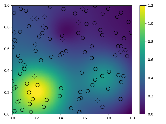
Interpolating scattered observations of Franke's test function with RBFs.
'''
import numpy as np
from rbf.interpolate import RBFInterpolant
import matplotlib.pyplot as plt
np.random.seed(1)
def frankes_test_function(x):
'''A commonly used test function for interpolation'''
x1, x2 = x[:, 0], x[:, 1]
term1 = 0.75 * np.exp(-(9*x1-2)**2/4 - (9*x2-2)**2/4)
term2 = 0.75 * np.exp(-(9*x1+1)**2/49 - (9*x2+1)/10)
term3 = 0.5 * np.exp(-(9*x1-7)**2/4 - (9*x2-3)**2/4)
term4 = -0.2 * np.exp(-(9*x1-4)**2 - (9*x2-7)**2)
y = term1 + term2 + term3 + term4
return y
# observation points
x_obs = np.random.random((100, 2))
# values at the observation points
u_obs = frankes_test_function(x_obs)
# evaluation points
x_itp = np.mgrid[0:1:200j, 0:1:200j].reshape(2, -1).T
interp = RBFInterpolant(x_obs, u_obs)
# interpolated values at the evaluation points
u_itp = interp(x_itp)
# plot the results
plt.tripcolor(
x_itp[:, 0], x_itp[:, 1], u_itp, cmap='viridis', vmin=0.0, vmax=1.2
)
plt.scatter(
x_obs[:, 0], x_obs[:, 1], s=100, c=u_obs, cmap='viridis', vmin=0.0,
vmax=1.2, edgecolor='k'
)
plt.xlim(0, 1)
plt.ylim(0, 1)
plt.colorbar()
plt.tight_layout()
plt.savefig('../figures/interpolate.f.png')
plt.show()
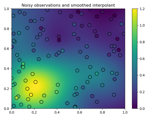
'''
Interpolating noisy scattered observations of Franke's test function with
smoothed RBFs.
'''
import numpy as np
from rbf.interpolate import RBFInterpolant
import matplotlib.pyplot as plt
import logging
logging.basicConfig(level=logging.INFO)
np.random.seed(1)
def frankes_test_function(x):
'''A commonly used test function for interpolation'''
x1, x2 = x[:, 0], x[:, 1]
term1 = 0.75 * np.exp(-(9*x1-2)**2/4 - (9*x2-2)**2/4)
term2 = 0.75 * np.exp(-(9*x1+1)**2/49 - (9*x2+1)/10)
term3 = 0.5 * np.exp(-(9*x1-7)**2/4 - (9*x2-3)**2/4)
term4 = -0.2 * np.exp(-(9*x1-4)**2 - (9*x2-7)**2)
y = term1 + term2 + term3 + term4
return y
# observation points
x_obs = np.random.random((100, 2))
# noisy values at the observation points
u_obs = frankes_test_function(x_obs) + np.random.normal(0.0, 0.1, (100,))
# evaluation points
x_itp = np.mgrid[0:1:200j, 0:1:200j].reshape(2, -1).T
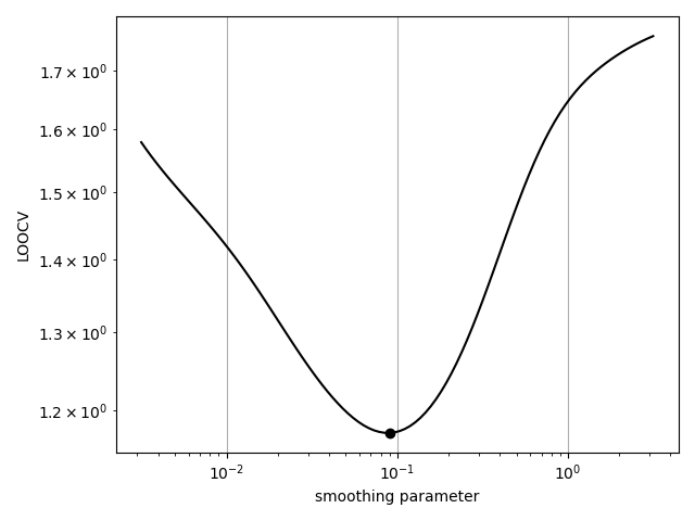
# automatically select a smoothing parameter that minimizes the leave-one-out
# cross validation (LOOCV) score.
interp = RBFInterpolant(x_obs, u_obs, sigma='auto')
# interpolated values at the evaluation points
u_itp = interp(x_itp)
# We could also minimize the LOOCV score ourselves with the `loocv` method.
# This may be helpful for better exploring the objective function.
sigmas = 10**np.linspace(-2.5, 0.5, 100)
loocvs = [RBFInterpolant.loocv(x_obs, u_obs, sigma=s) for s in sigmas]
opt_sigma = sigmas[np.argmin(loocvs)]
print('optimal sigma: %s' % opt_sigma)
# plot the results
plt.figure(1)
plt.tripcolor(
x_itp[:, 0], x_itp[:, 1], u_itp, cmap='viridis', vmin=0.0, vmax=1.2
)
plt.scatter(
x_obs[:, 0], x_obs[:, 1], s=100, c=u_obs, cmap='viridis', vmin=0.0,
vmax=1.2, edgecolor='k'
)
plt.xlim(0, 1)
plt.ylim(0, 1)
plt.colorbar()
plt.title('Noisy observations and smoothed interpolant')
plt.tight_layout()
plt.savefig('../figures/interpolate.g.1.png')
plt.figure(2)
plt.loglog(sigmas, loocvs, 'k-')
plt.plot([opt_sigma], [np.min(loocvs)], 'ko')
plt.grid()
plt.xlabel('smoothing parameter')
plt.ylabel('LOOCV')
plt.tight_layout()
plt.savefig('../figures/interpolate.g.2.png')
plt.show()
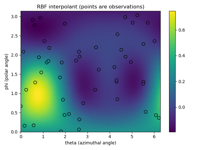
'''
RBF Interpolation on a unit sphere. This is done by converting theta
(azimuthal angle) and phi (polar angle) into cartesian coordinates and
then interpolating over R^3.
'''
import numpy as np
from rbf.interpolate import RBFInterpolant
import matplotlib.pyplot as plt
np.random.seed(1)
def spherical_to_cartesian(theta, phi):
x = np.sin(phi)*np.cos(theta)
y = np.sin(phi)*np.sin(theta)
z = np.cos(phi)
return np.array([x, y, z]).T
def true_function(theta, phi):
# create some arbitary function that we want to recontruct with
# interpolation
cart = spherical_to_cartesian(theta, phi)
out = (np.cos(cart[:, 2] - 1.0)*
np.cos(cart[:, 0] - 1.0)*
np.cos(cart[:, 1] - 1.0))
return out
# number of observation points
nobs = 50
# make the observation points in spherical coordinates
theta_obs = np.random.uniform(0.0, 2*np.pi, nobs)
phi_obs = np.random.uniform(0.0, np.pi, nobs)
# get the cartesian coordinates for the observation points
cart_obs = spherical_to_cartesian(theta_obs, phi_obs)
# get the latent function at the observation points
val_obs = true_function(theta_obs, phi_obs)
# make a grid of interpolation points in spherical coordinates
theta_itp, phi_itp = np.meshgrid(np.linspace(0.0, 2*np.pi, 100),
np.linspace(0.0, np.pi, 100))
theta_itp = theta_itp.flatten()
phi_itp = phi_itp.flatten()
# get the catesian coordinates for the interpolation points
cart_itp = spherical_to_cartesian(theta_itp, phi_itp)
# create an RBF interpolant from the cartesian observation points. I
# am just use the default `RBFInterpolant` parameters here, nothing
# special.
I = RBFInterpolant(cart_obs, val_obs)
# evaluate the interpolant on the interpolation points
val_itp = I(cart_itp)
## PLOTTING
# plot the interpolant in spherical coordinates
plt.figure(1)
plt.title('RBF interpolant (points are observations)')
# plot the interpolated function
p = plt.tripcolor(theta_itp, phi_itp, val_itp,
cmap='viridis')
# plot the observations
plt.scatter(theta_obs, phi_obs, c=val_obs,
s=50, edgecolor='k', cmap='viridis',
vmin=p.get_clim()[0], vmax=p.get_clim()[1])
plt.colorbar(p)
plt.xlabel('theta (azimuthal angle)')
plt.ylabel('phi (polar angle)')
plt.xlim(0, 2*np.pi)
plt.ylim(0, np.pi)
plt.grid()
plt.grid(ls=':', color='k')
plt.tight_layout()
plt.savefig('../figures/interpolate.b.1.png')
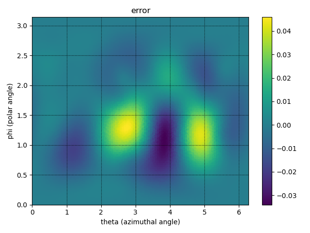
# plot the true function in spherical coordinates
val_true = true_function(theta_itp, phi_itp)
plt.figure(2)
plt.title('error')
p = plt.tripcolor(theta_itp, phi_itp, val_itp - val_true,
cmap='viridis')
plt.colorbar(p)
plt.xlabel('theta (azimuthal angle)')
plt.ylabel('phi (polar angle)')
plt.xlim(0, 2*np.pi)
plt.ylim(0, np.pi)
plt.grid(ls=':', color='k')
plt.tight_layout()
plt.savefig('../figures/interpolate.b.2.png')
# compute and print the mean L2 error
mean_error = np.mean(np.abs(val_true - val_itp))
print('mean interpolation error: %s' % mean_error)
plt.show()
'''
This script compares RBFInterpolant to NearestRBFInterpolant class for Franke's
test function.
'''
import numpy as np
import matplotlib.pyplot as plt
from rbf.interpolate import RBFInterpolant, KNearestRBFInterpolant
np.random.seed(1)
def frankes_test_function(x):
x1, x2 = x[:, 0], x[:, 1]
term1 = 0.75 * np.exp(-(9*x1-2)**2/4 - (9*x2-2)**2/4)
term2 = 0.75 * np.exp(-(9*x1+1)**2/49 - (9*x2+1)/10)
term3 = 0.5 * np.exp(-(9*x1-7)**2/4 - (9*x2-3)**2/4)
term4 = -0.2 * np.exp(-(9*x1-4)**2 - (9*x2-7)**2)
y = term1 + term2 + term3 + term4
return y
# the observations and their locations for interpolation
xobs = np.random.uniform(0.0, 1.0, (500, 2))
yobs = frankes_test_function(xobs)
# the locations where we evaluate the interpolants
xitp = np.mgrid[0:1:200j, 0:1:200j].reshape(2, -1).T
# the true function which we want the interpolants to reproduce
true_soln = frankes_test_function(xitp)
yitp = RBFInterpolant(xobs, yobs)(xitp)
fig, ax = plt.subplots(1, 2, figsize=(9, 3.5))
ax[0].set_title('RBFInterpolant')
p = ax[0].tripcolor(xitp[:, 0], xitp[:, 1], yitp)
ax[0].scatter(xobs[:, 0], xobs[:, 1], c='k', s=3)
ax[0].set_xlim(0, 1)
ax[0].set_ylim(0, 1)
ax[0].set_aspect('equal')
ax[0].grid(ls=':', color='k')
fig.colorbar(p, ax=ax[0])
ax[1].set_title('|error|')
p = ax[1].tripcolor(xitp[:, 0], xitp[:, 1], np.abs(yitp - true_soln))
ax[1].set_xlim(0, 1)
ax[1].set_ylim(0, 1)
ax[1].set_aspect('equal')
ax[1].grid(ls=':', color='k')
fig.colorbar(p, ax=ax[1])
fig.tight_layout()
plt.savefig('../figures/interpolate.c.all.png')
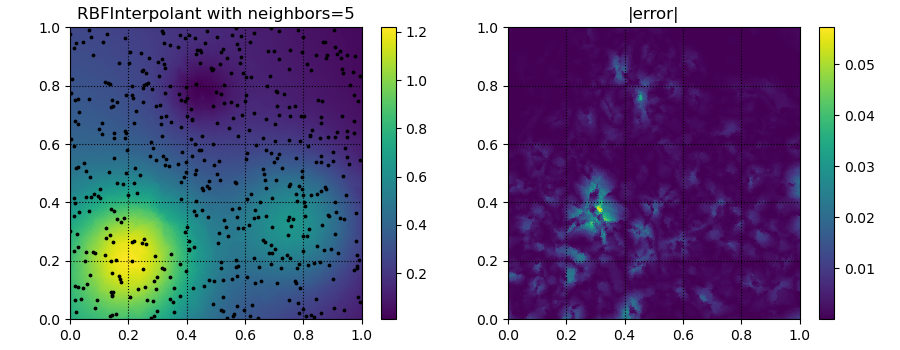
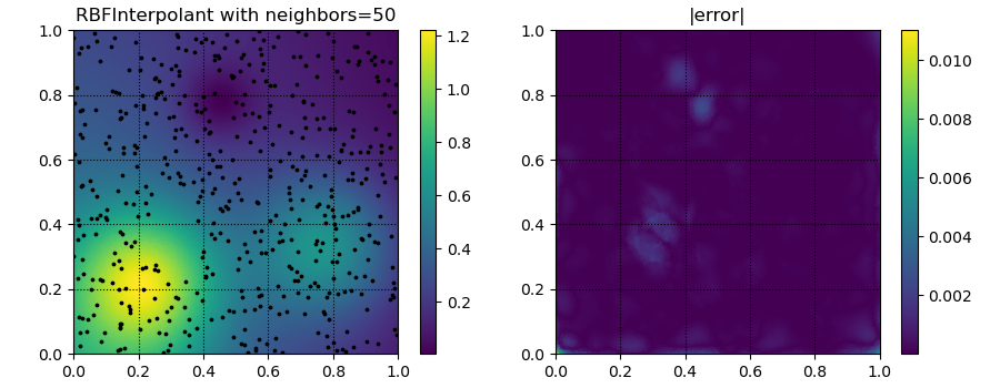
for k in [5, 20, 50]:
yitp = RBFInterpolant(xobs, yobs, neighbors=k)(xitp)
fig, ax = plt.subplots(1, 2, figsize=(9, 3.5))
ax[0].set_title('RBFInterpolant with neighbors=%d' % k)
p = ax[0].tripcolor(xitp[:, 0], xitp[:, 1], yitp)
ax[0].scatter(xobs[:, 0], xobs[:, 1], c='k', s=3)
ax[0].set_xlim(0, 1)
ax[0].set_ylim(0, 1)
ax[0].set_aspect('equal')
ax[0].grid(ls=':', color='k')
fig.colorbar(p, ax=ax[0])
ax[1].set_title('|error|')
p = ax[1].tripcolor(xitp[:, 0], xitp[:, 1], np.abs(yitp - true_soln))
ax[1].set_xlim(0, 1)
ax[1].set_ylim(0, 1)
ax[1].set_aspect('equal')
ax[1].grid(ls=':', color='k')
fig.colorbar(p, ax=ax[1])
fig.tight_layout()
plt.savefig('../figures/interpolate.c.%d.png' % k)
plt.show()