gproc (Gaussian Process)

This module defines the GaussianProcess class which is used to perform Gaussian process regression (GPR) and other operations with Gaussian processes. GPR is also known as Kriging or Least Squares Collocation. It is a technique for constructing a continuous function from discrete observations by incorporating a stochastic prior model for the underlying function.

There are several existing python packages for Gaussian processes (See www.gaussianprocess.org for an updated list of packages). This module was written because existing software lacked support for 1) Gaussian processes with added basis functions 2) analytical differentiation of Gaussian processes and 3) conditioning a Gaussian process with derivative constraints. Other software packages have a strong focus on optimizing hyperparameters based on data likelihood. This module does not include any optimization routines and hyperparameters are always explicitly specified by the user. However, the GaussianProcess class contains the log_likelihood method which can be used along with functions from scipy.optimize to optimize hyperparameters.

Gaussian processes

To understand what a Gaussian process is, let’s first consider a random vector \(\mathbf{u}\) which has a multivariate normal distribution with mean \(\bar{\mathbf{u}}\) and covariance matrix \(\mathbf{C}\). That is to say, each element \(u_i\) of \(\mathbf{u}\) is a normally distributed random variable with mean \(\bar{u}_i\) and covariance \(C_{ij}\) with element \(u_j\). Each element also has context (e.g., time or position) denoted as \(x_i\). A Gaussian process is the continuous analogue to the multivariate normal vector, where the context for a Gaussian process is a continuous variable \(x\), rather than the discrete variable \(x_i\). A Gaussian process \(u_o\) is defined in terms of a mean function \(\bar{u}\), and a covariance function \(C_u\). We write this definition of \(u_o\) more concisely as

\[u_o \sim \mathcal{GP}\left(\bar{u},C_u\right).\]

Analogous to each element of the random vector \(\mathbf{u}\), the Gaussian process at \(x\), denoted as \(u_o(x)\), is a normally distributed random variable with mean \(\bar{u}(x)\) and covariance \(C_u(x, x')\) with \(u_o(x')\).

In this module, we adopt a more general definition of a Gaussian process by incorporating basis functions. These basis functions are added to Gaussian processes to account for arbitrary shifts or trends in the data that we are trying to model. To be more precise, we consider a Gaussian process \(u(x)\) to be the combination of \(u_o(x)\), a proper Gaussian process, and a set of \(m\) basis functions, \(\mathbf{p}_u(x) = \{p_i(x)\}_{i=1}^m\), whose coefficients, \(\{c_i\}_{i=1}^m\), are completely unknown (i.e., they have infinite variance). We then express \(u(x)\) as

\[u(x) = u_o(x) + \sum_{i=1}^m c_i p_i(x).\]

When we include these basis functions, the Gaussian process \(u(x)\) becomes improper because it has infinite variance. So when we refer to the covariance function for a Gaussian process \(u(x)\), we are actually referring to the covariance function for its proper component \(u_o(x)\).

Throughout this module we will define a Gaussian process u(x) in terms of its mean function \(\bar{u}(x)\), its covariance function \(C_u(x, x')\), as well as its basis functions \(\mathbf{p}_u(x)\).

Operations on Gaussian processes

Gaussian processes can be constructed from other Gaussian processes. There are four implemented operations on Gaussian processes that result in a new Gaussian process: addition, scaling, differentiation, and conditioning.

Addition

Two uncorrelated Gaussian processes, \(u\) and \(v\), can be added as

\[u(x) + v(x) = z(x)\]

where the mean, covariance, and basis functions for \(z\) are

\[\bar{z}(x) = \bar{u}(x) + \bar{v}(x),\]

\[C_z(x,x') = C_u(x,x') + C_v(x,x'),\]

and

\[\mathbf{p}_z(x) = \mathbf{p}_u(x) \cup \mathbf{p}_v(x).\]

Scaling

A Gaussian process can be scaled by a constant as

\[cu(x) = z(x)\]

where

\[\bar{z}(x) = c\bar{u}(x),\]

\[C_z(x,x') = c^2C_u(x,x'),\]

and

\[\mathbf{p}_z(x) = \mathbf{p}_u(x).\]

Differentiation

A Gaussian process can be differentiated with respect to \(x_i\) as

\[\frac{\partial}{\partial x_i} u(x) = z(x),\]

where

\[\bar{z}(x) = \frac{\partial}{\partial x_i}\bar{u}(x),\]

\[C_z(x,x') = \frac{\partial^2}{\partial x_i \partial x_i'} C_u(x,x'),\]

and

\[\mathbf{p}_z(x) = \left\{\frac{\partial}{\partial x_i} p_k(x) \mid p_k(x) \in \mathbf{p}_u(x)\right\}\]

Conditioning

A Gaussian process can be conditioned with \(q\) noisy observations of \(u(x)\), \(\mathbf{d}=\{d_i\}_{i=1}^q\), which have been made at locations \(\mathbf{y}=\{y_i\}_{i=1}^q\). These observations have noise with zero mean and covariance described by \(\mathbf{C_d}\). The conditioned Gaussian process is

\[u(x) | \mathbf{d} = z(x)\]

where

\[\bar{z}(x) = \bar{u}(x) + \mathbf{k}(x,\mathbf{y}) \mathbf{K}(\mathbf{y})^{-1} \mathbf{r},\]

\[C_{z}(x,x') = C_u(x,x') - \mathbf{k}(x,\mathbf{y}) \mathbf{K}(\mathbf{y})^{-1} \mathbf{k}(x',\mathbf{y})^T,\]

and

\[\mathbf{p}_z(x) = \emptyset.\]

In the above equations we use the augmented covariance matrices, \(\mathbf{k}\) and \(\mathbf{K}\), whose entries are

\[\begin{split}\mathbf{k}(x,\mathbf{y}) = \left[ \begin{array}{cc} \left[C_u(x,y_i)\right]_{y_i \in \mathbf{y}} & \mathbf{p}_u(x) \\ \end{array} \right]\end{split}\]

and

\[\begin{split}\mathbf{K}(\mathbf{y}) = \left[ \begin{array}{cc} \mathbf{C_d} + \left[C_u(y_i,y_j)\right]_ {y_i,y_j \in \mathbf{y}\times\mathbf{y}} & [\mathbf{p}_u(y_i)]_{y_i \in \mathbf{y}} \\ [\mathbf{p}_u(y_i)]^T_{y_i \in \mathbf{y}} & \mathbf{0} \\ \end{array} \right].\end{split}\]

We also used the residual vector, \(\mathbf{r}\), whose entries are

\[\begin{split}\mathbf{r} = \left[ \begin{array}{c} \left([d_i - \bar{u}(y_i)]_{i=1}^q\right)^T \\ \mathbf{0} \end{array} \right].\end{split}\]

Note that there are no basis functions in \(z\) because it is assumed that there is enough data in \(\mathbf{d}\) to constrain the basis functions in \(u\). If \(\mathbf{d}\) is not sufficiently informative then \(\mathbf{K}(\mathbf{y})\) will not be invertible. A necessary but not sufficient condition for \(\mathbf{K}(\mathbf{y})\) to be invertible is that \(q \geq m\).

Some commonly used Gaussian processes

The GaussianProcess class is quite general as it can be instantiated with any user-specified mean function, covariance function, or set of basis functions. However, supplying these requisite functions can be laborious. This module contains several constructors to simplify instantiating some commonly used types of Gaussian processes. The types of Gaussian processes which have constructors are listed below.

Isotropic Gaussian Processes

An isotropic Gaussian process has zero mean and a covariance function which can be written as a function of \(r = ||x - x'||_2\) and a shape parameters \(\epsilon\),

\[C_u(x,x') = \sigma^2 \phi(r\ ; \epsilon),\]

where \(\phi(r\ ; \epsilon)\) is a positive definite radial basis function. One common choice for \(\phi\) is the squared exponential function,

\[\phi(r\ ;\epsilon) = \exp\left(\frac{-r^2}{\epsilon^2}\right),\]

which has the useful property of being infinitely differentiable.

An instance of a GaussianProcess with an isotropic covariance function can be created with the function gpiso.

Gaussian Process with a Gibbs covariance function

A Gaussian process with a Gibbs covariance function is useful because, unlike for isotropic Gaussian processes, it can have a spatially variable lengthscale. Given some user-specified lengthscale function \(\ell_d(x)\), which gives the lengthscale at \(x \in \mathbb{R}^D\) along dimension \(d\), the Gibbs covariance function is

\[C_u(x, x') = \sigma^2 \prod_{d=1}^D \left( \frac{2 \ell_d(x) \ell_d(x')}{\ell_d(x)^2 + \ell_d(x')^2} \right)^{1/2} \exp\left(-\sum_{d=1}^D \frac{(x_d - x_d')^2}{\ell_d(x)^2 + \ell_d(x')^2} \right).\]

An instance of a GaussianProcess with a Gibbs covariance function can be created with the function gpgibbs.

Gaussian Process with mononomial basis functions

Polynomials are often added to Gaussian processes to improve their ability to describe offsets and trends in data. The function gppoly is used to create a GaussianProcess with zero mean, zero covariance, and a set of monomial basis function that span the space of all polynomials with some degree, \(d\). For example, if \(x \in \mathbb{R}^2\) and \(d=1\), then the monomial basis functions would be

\[\mathbf{p}_u(x) = \{1,x_1,x_2\}.\]

Examples

Here we provide a basic example that demonstrates creating a GaussianProcess and performing GPR. Suppose we have 5 scalar valued observations d that were made at locations x, and we want interpolate these observations with GPR

>>> x = [[0.0], [1.0], [2.0], [3.0], [4.0]]
>>> d = [2.3, 2.2, 1.7, 1.8, 2.4]

First we define our prior for the underlying function that we want to interpolate. We assume an isotropic GaussianProcess with a squared exponential covariance function and the parameters \(\sigma^2=1.0\) and \(\epsilon=0.5\).

>>> from rbf.gproc import gpiso
>>> gp_prior = gpiso('se', eps=0.5, var=1.0)

We also want to include an unknown constant offset to our prior model, which is done with the command

>>> from rbf.gproc import gppoly
>>> gp_prior += gppoly(0)

Now we condition the prior with the observations to form the posterior

>>> gp_post = gp_prior.condition(x, d)

We can now evaluate the mean and covariance of the posterior anywhere using the mean or covariance method. We can also evaluate just the mean and standard deviation by calling the instance

>>> m, s = gp_post([[0.5], [1.5], [2.5], [3.5]])

References

[1] Rasmussen, C., and Williams, C., Gaussian Processes for Machine Learning. The MIT Press, 2006.

class rbf.gproc.GaussianProcess(mean=None, covariance=None, basis=None, variance=None, dim=None, differentiable=False)

Bases: object

Class for performing basic operations with Gaussian processes. A Gaussian process is stochastic process defined by a mean function, a covariance function, and a set of basis functions.

Parameters:

mean (callable, optional) – Function that takes an (N, D) float array of points as input and returns the mean of the Gaussian process at those points. If differentiable is True, the functions should also take a (D,) int array of derivative specifications as a second argument.
covariance (callable, optional) – Function that takes an (N, D) float array and an (M, D) float array of points as input and returns the covariance of the Gaussian process between those points as an (N, M) array or sparse matrix. If differentiable is True, the functions should also take two (D,) int array of derivative specifications as a third and fourth argument.
basis (callable, optional) – Function that takes an (N, D) float array of points as input and returns the basis functions evaluated at those points. If differentiable is True, the functions should also take a (D,) int array of derivative specifications as a second argument.
variance (callable, optional) – Function that takes an (N, D) float array of points as input and returns the variance of the Gaussian process at those points. If differentiable is True, the functions should also take a (D,) int array of derivative specifications as a second argument.
dim (int, optional) – Fixes the spatial dimensions of the GaussianProcess instance. An error will be raised if method arguments have a conflicting number of spatial dimensions.
differentiable (bool, optional) – Whether the GaussianProcess is differentiable. If True, the provided mean, covariance, basis, and variance functions are expected to take derivative specifications as input.

Examples

Create a GaussianProcess describing Brownian motion

>>> import numpy as np
>>> from rbf.gauss import GaussianProcess
>>> def mean(x): return np.zeros(x.shape[0])
>>> def cov(x1, x2): return np.minimum(x1[:, None, 0], x2[None, :, 0])
>>> gp = GaussianProcess(mean, cov, dim=1) # Brownian motion is 1D

__add__(other): Equivalent to calling add.

__call__(x, chunk_size=100)

Returns the mean and standard deviation of the Gaussian process.

Parameters:

x ((N, D) array) – Evaluation points.
chunk_size (int, optional) – Break x into chunks with this size for evaluation.

Returns:

(N,) array – Mean at x.
(N,) array – One standard deviation at x.

__mul__(c): Equivalent to calling scale.

__sub__(other): Equivalent to calling subtract.

add(other): Adds two GaussianProcess instances.

basis(x, diff=None)

Returns the basis functions evaluated at x.

Parameters:

x ((N, D) array) – Evaluation points.
diff ((D,) int array) – Derivative specification.

Returns:

(N, P) array

condition(y, d, dcov=None, dvecs=None, ddiff=None, build_inverse=False)

Returns a GaussianProcess conditioned on the data.

Parameters:

y ((N, D) float array) – Observation points.
d ((N,) float array) – Observed values at y.
dcov ((N, N) array or sparse matrix, optional) – Covariance of the data noise. Defaults to a dense array of zeros.
dvecs ((N, P) array, optional) – Data noise basis vectors. The data noise is assumed to contain some unknown linear combination of the columns of dvecs.
ddiff ((D,) int array, optional) – Derivative of the observations. For example, use (1,) if the observations are 1-D and should constrain the slope.
build_inverse (bool, optional) – Whether to construct the inverse matrices rather than just the factors.

Returns:

GaussianProcess

covariance(x1, x2, diff1=None, diff2=None)

Returns the covariance matrix of the Gaussian process.

Parameters:

x2 (x1,) – Evaluation points.
diff2 (diff1,) – Derivative specifications.

Returns:

(N, M) array or sparse matrix

differentiate(d): Returns a differentiated GaussianProcess.

is_positive_definite(x): Tests if the covariance function evaluated at x is positive definite.

log_likelihood(y, d, dcov=None, dvecs=None)

Returns the log likelihood of drawing the observations d from the Gaussian process. The observations could potentially have noise which is described by dcov and dvecs. If the Gaussian process contains any basis functions or if dvecs is specified, then the restricted log likelihood is returned.

Parameters:

y ((N, D) array) – Observation points.
d ((N,) array) – Observed values at y.
dcov ((N, N) array or sparse matrix, optional) – Data covariance. If not given, this will be a dense matrix of zeros.
dvecs ((N, P) float array, optional) – Basis vectors for the noise. The data noise is assumed to contain some unknown linear combination of the columns of dvecs.

Returns:

float

mean(x, diff=None)

Returns the mean of the Gaussian process.

Parameters:

x ((N, D) array) – Evaluation points.
diff ((D,) int array) – Derivative specification.

Returns:

(N,) array

outliers(x, d, dsigma, tol=4.0, maxitr=50)

Identifies values in d that are abnormally inconsistent with the the Gaussian process

Parameters:

x ((N, D) float array) – Observations locations.
d ((N,) float array) – Observations.
dsigma ((N,) float array) – One standard deviation uncertainty on the observations.
tol (float, optional) – Outlier tolerance. Smaller values make the algorithm more likely to identify outliers. A good value is 4.0 and this should not be set any lower than 2.0.
maxitr (int, optional) – Maximum number of iterations.

Returns:

(N,) bool array – Array indicating which data are outliers

sample(x, use_cholesky=False, count=None): Draws a random sample from the Gaussian process.

scale(c): Returns a scaled GaussianProcess.

subtract(other): Subtracts two GaussianProcess instances.

variance(x, diff=None)

Returns the variance of the Gaussian process.

Parameters:

x ((N, D) array) – Evaluation points.
diff ((D,) int array) – Derivative specification.

Returns:

(N,) array

rbf.gproc.covariance_differentiator(delta)

Decorator that makes a covariance function differentiable. The derivatives are approximated by finite differences. The function must take an (N, D) array and an (M, D) array of positions as input. The returned function takes an (N, D) array and an (M, D) array of positions and two (D,) array derivative specifications.

Parameters:: delta (float) – step size to use for finite differences

rbf.gproc.differentiator(delta)

Decorator that makes a function differentiable. The derivatives of the function are approximated by finite differences. The function must take a single (N, D) array of positions as input. The returned function takes a single (N, D) array of positions and a (D,) array derivative specification.

Parameters:: delta (float) – step size to use for finite differences

rbf.gproc.empty_basis(x, diff): Empty set of basis functions.

rbf.gproc.gpgibbs(lengthscale, sigma, delta=0.0001)

Returns a Gaussian process with a Gibbs covariance function. The Gibbs kernel has a spatially varying lengthscale.

Parameters:

lengthscale (function) – Function that takes an (N, D) array of positions and returns an (N, D) array indicating the lengthscale along each dimension at those positions.
sigma (float) – Standard deviation of the Gaussian process.
delta (float, optional) – Finite difference spacing to use when calculating the derivative of the GaussianProcess. An analytical solution for the derivative is not available because the derivative of the lengthscale function is unknown.

Returns:

GaussianProcess

rbf.gproc.gpiso(phi, eps, var, dim=None)

Creates an isotropic Gaussian process which has a covariance function that is described by a radial basis function.

Parameters:

phi (str or RBF instance) – Radial basis function describing the covariance function.
eps (float) – Shape parameter.
var (float) – Variance.
dim (int, optional) – Fixes the spatial dimensions of the domain.

Returns:

GaussianProcess

Notes

Not all radial basis functions are positive definite, which means that it is possible to instantiate an invalid GaussianProcess. The method is_positive_definite provides a necessary but not sufficient test for positive definiteness. Examples of predefined RBF instances which are positive definite include: rbf.basis.se, rbf.basis.ga, rbf.basis.exp, rbf.basis.iq, rbf.basis.imq.

rbf.gproc.gppoly(order, dim=None)

Returns a Gaussian process consisting of monomial basis functions.

Parameters:

order (int) – Order of the polynomial spanned by the basis functions.
dim (int, optional) – Fixes the spatial dimensions of the domain.

Returns:

GaussianProcess

rbf.gproc.log_likelihood(d, mu, cov, vecs=None)

Returns the log likelihood of observing d from a multivariate normal distribution with mean mu and covariance cov.

When vecs is specified, the restricted log likelihood is returned. The restricted log likelihood is the probability of observing R.dot(d) from a normally distributed random vector with mean R.dot(mu) and covariance R.dot(sigma).dot(R.T), where R is a matrix with rows that are orthogonal to the columns of vecs. See [1] or [2] for more information.

Parameters:

d ((N,) array) – Observation vector.
mu ((N,) array) – Mean vector.
cov ((N, N) array or sparse matrix) – Covariance matrix.
vecs ((N, M) array, optional) – Unconstrained basis vectors.

Returns:

float

References

[1] Harville D. (1974). Bayesian Inference of Variance Components Using Only Error Contrasts. Biometrica.

[2] Cressie N. (1993). Statistics for Spatial Data. John Wiley & Sons.

rbf.gproc.naive_variance_constructor(covariance): Converts a covariance function to a variance function.

rbf.gproc.outliers(d, dsigma, pcov, pmu=None, pvecs=None, tol=4.0, maxitr=50)

Uses a data editing algorithm to identify outliers in d. Outliers are considered to be the data that are abnormally inconsistent with a multivariate normal distribution with mean pmu, covariance pcov, and basis vectors pvecs.

The data editing algorithm first conditions the prior with the observations, then it compares each residual (d minus the expected value of the posterior divided by dsigma) to the RMS of residuals. Data with residuals greater than tol times the RMS are identified as outliers. This process is then repeated using the subset of d which were not flagged as outliers. If no new outliers are detected in an iteration then the algorithm stops.

Parameters:

d ((N,) float array) – Observations.
dsigma ((N,) float array) – One standard deviation uncertainty on the observations.
pcov ((N, N) array or sparse matrix) – Covariance of the prior at the observation points.
pmu ((N,) float array, optional) – Mean of the prior at the observation points. Defaults to zeros.
pvecs ((N, P) float array, optional) – Basis functions of the prior evaluated at the observation points. Defaults to an (N, 0) array.
tol (float, optional) – Outlier tolerance. Smaller values make the algorithm more likely to identify outliers. A good value is 4.0 and this should not be set any lower than 2.0.
maxitr (int, optional) – Maximum number of iterations.

Returns:

(N,) bool array – Array indicating which data are outliers

rbf.gproc.sample(mu, cov, use_cholesky=False, count=None)

Draws a random sample from the multivariate normal distribution.

Parameters:

mu ((N,) array) – Mean vector.
cov ((N, N) array or sparse matrix) – Covariance matrix.
use_cholesky (bool, optional) – Whether to use the Cholesky decomposition or eigenvalue decomposition. The former is faster but fails when cov is not numerically positive definite.
count (int, optional) – Number of samples to draw.

Returns:

(N,) or (count, N) array

rbf.gproc.zero_covariance(x1, x2, diff1, diff2): Covariance function that returns zeros.

rbf.gproc.zero_mean(x, diff): Mean function that returns zeros.

rbf.gproc.zero_variance(x, diff): Variance function that returns zeros.

Examples

''' 
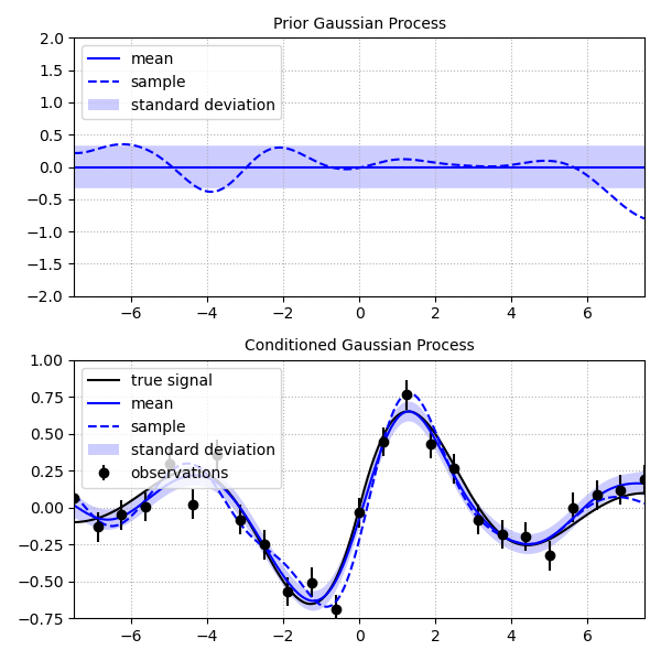
This script demonstrates how to perform Gaussian process regression on a noisy
data set. It also demonstrates drawing samples of the prior and posterior to
provide the user with an intuitive understanding of their distributions.
'''
import logging
import numpy as np
import matplotlib.pyplot as plt
from scipy.optimize import minimize

from rbf.gproc import gpiso

logging.basicConfig(level=logging.DEBUG)
np.random.seed(1)

# observation points
y = np.linspace(-7.5, 7.5, 25) 
# interpolation points
x = np.linspace(-7.5, 7.5, 1000) 
# true signal
u_true = np.exp(-0.3*np.abs(x))*np.sin(x)
# observation noise covariance
dsigma = np.full(25, 0.1)
dcov = np.diag(dsigma**2)
# noisy observations of the signal
d = np.exp(-0.3*np.abs(y))*np.sin(y) + np.random.normal(0.0, dsigma)

def negative_log_likelihood(params):
    log_eps, log_var = params
    gp = gpiso('se', eps=10**log_eps, var=10**log_var) 
    out = -gp.log_likelihood(y[:, None], d, dcov=dcov)
    return out

log_eps, log_var = minimize(negative_log_likelihood, [0.0, 0.0]).x
# create a prior GaussianProcess using the most likely variance and lengthscale
gp_prior = gpiso('se', eps=10**log_eps, var=10**log_var)
# generate a sample of the prior
sample_prior = gp_prior.sample(x[:, None]) 
# find the mean and standard deviation of the prior
mean_prior, std_prior = gp_prior(x[:, None])
# condition the prior on the observations
gp_post = gp_prior.condition(y[:, None], d, dcov=dcov)
sample_post = gp_post.sample(x[:, None]) 
mean_post, std_post = gp_post(x[:, None])

## Plotting
#####################################################################
fig, axs = plt.subplots(2, 1, figsize=(6, 6))
ax = axs[0]
ax.grid(ls=':')
ax.tick_params(labelsize=10)
ax.set_title('Prior Gaussian Process', fontsize=10)
ax.plot(x, mean_prior, 'b-', label='mean')
ax.fill_between(x, mean_prior - std_prior, mean_prior + std_prior, color='b',
                alpha=0.2, edgecolor='none', label='standard deviation')

ax.plot(x, sample_prior, 'b--', label='sample')
ax.set_xlim((-7.5, 7.5))
ax.set_ylim((-2.0, 2.0))
ax.legend(loc=2, fontsize=10)
ax = axs[1]
ax.grid(ls=':')
ax.tick_params(labelsize=10)
ax.set_title('Conditioned Gaussian Process', fontsize=10)
ax.errorbar(y, d, dsigma, fmt='ko', capsize=0, label='observations')
ax.plot(x, u_true, 'k-', label='true signal')
ax.plot(x, mean_post, 'b-', label='mean')
ax.plot(x, sample_post, 'b--', label='sample')
ax.fill_between(x, mean_post-std_post, mean_post+std_post, color='b',
                alpha=0.2, edgecolor='none', label='standard deviation')
ax.set_xlim((-7.5, 7.5))
ax.set_ylim((-0.75, 1.0))
ax.legend(loc=2, fontsize=10)
plt.tight_layout()
plt.savefig('../figures/gproc.a.png')
plt.show()

''' 
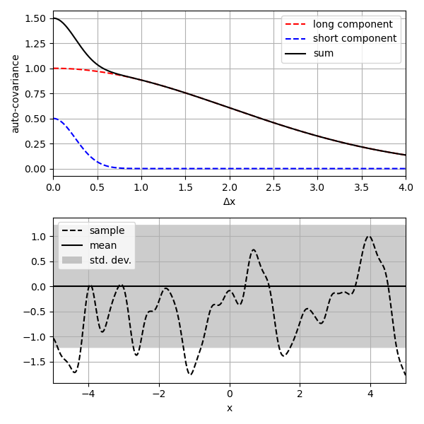
This script demonstrates how to make a custom *GaussianProcess* by 
combining *GaussianProcess* instances. The resulting Gaussian process 
has two distinct length-scales.
'''
import numpy as np
import matplotlib.pyplot as plt
from rbf.gproc import gpiso
np.random.seed(1)

dx = np.linspace(0.0, 5.0, 1000)[:, None]
x = np.linspace(-5, 5.0, 1000)[:, None]
gp_long = gpiso('se', eps=2.0, var=1.0)
gp_short = gpiso('se', eps=0.25, var=0.5)
gp = gp_long + gp_short
# compute the autocovariances 
acov_long = gp_long.covariance(dx, [[0.0]])
acov_short = gp_short.covariance(dx, [[0.0]])
acov = gp.covariance(dx, [[0.0]])
# draw 3 samples
sample = gp.sample(x) 
# mean and uncertainty of the new gp
mean, sigma = gp(x)
# plot the autocovariance functions
fig, axs = plt.subplots(2, 1, figsize=(6, 6))
axs[0].plot(dx, acov_long, 'r--', label='long component')
axs[0].plot(dx, acov_short, 'b--', label='short component')
axs[0].plot(dx, acov, 'k-', label='sum')
axs[0].set_xlabel('$\mathregular{\Delta x}$', fontsize=10)
axs[0].set_ylabel('auto-covariance', fontsize=10)
axs[0].legend(fontsize=10)
axs[0].tick_params(labelsize=10)
axs[0].set_xlim((0, 4))
axs[0].grid(True)
# plot the samples
axs[1].plot(x, sample, 'k--', label='sample') 
axs[1].plot(x, mean, 'k-', label='mean')
axs[1].fill_between(x[:, 0], mean-sigma, mean+sigma, color='k', alpha=0.2, edgecolor='none', label='std. dev.')
axs[1].set_xlabel('x', fontsize=10)
axs[1].legend(fontsize=10)
axs[1].tick_params(labelsize=10)
axs[1].set_xlim((-5, 5))
axs[1].grid(True)
plt.tight_layout()
plt.savefig('../figures/gproc.b.png')
plt.show()

''' 
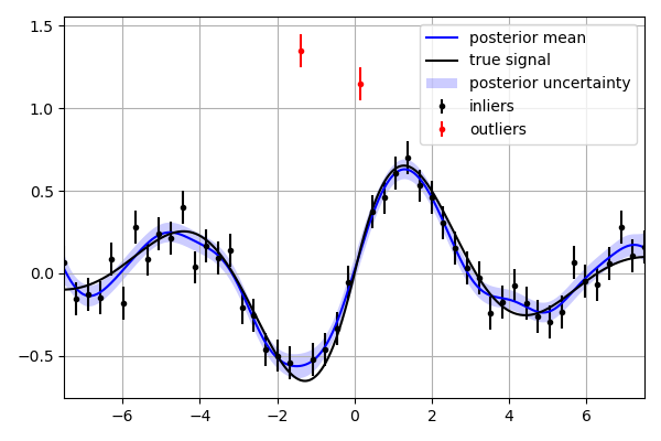
This script describes how to use the *outliers* method to detect and
remove outliers prior to conditioning a *GaussinaProcess*. 
'''
import numpy as np
import matplotlib.pyplot as plt
import logging
from rbf.gproc import gpiso, gppoly
logging.basicConfig(level=logging.DEBUG)
np.random.seed(1)

y = np.linspace(-7.5, 7.5, 50) # obsevation points
x = np.linspace(-7.5, 7.5, 1000) # interpolation points
truth = np.exp(-0.3*np.abs(x))*np.sin(x)  # true signal at interp. points
# form synthetic data
obs_sigma = np.full(50, 0.1) # noise standard deviation
noise = np.random.normal(0.0, obs_sigma)
noise[20], noise[25] = 2.0, 1.0 # add anomalously large noise
obs_mu = np.exp(-0.3*np.abs(y))*np.sin(y) + noise
# form prior Gaussian process
prior = gpiso('se', eps=1.0, var=1.0) + gppoly(1)
# find outliers which will be removed
toss = prior.outliers(y[:, None], obs_mu, obs_sigma, tol=4.0)
# condition with non-outliers
post = prior.condition(
    y[~toss, None],
    obs_mu[~toss],
    dcov=np.diag(obs_sigma[~toss]**2)
    )
post_mu, post_sigma = post(x[:, None])
# plot the results
fig, ax = plt.subplots(figsize=(6, 4)) 
ax.errorbar(y[~toss], obs_mu[~toss], obs_sigma[~toss], fmt='k.', capsize=0.0, label='inliers') 
ax.errorbar(y[toss], obs_mu[toss], obs_sigma[toss], fmt='r.', capsize=0.0, label='outliers') 
ax.plot(x, post_mu, 'b-', label='posterior mean') 
ax.fill_between(x, post_mu-post_sigma, post_mu+post_sigma, 
                color='b', alpha=0.2, edgecolor='none',
                label='posterior uncertainty') 
ax.plot(x, truth, 'k-', label='true signal') 
ax.legend(fontsize=10)
ax.set_xlim((-7.5, 7.5))
ax.grid(True)
fig.tight_layout()
plt.savefig('../figures/gproc.c.png')
plt.show()

''' 
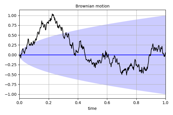
This script demonstrates how create a Gaussian process describing 
Brownian motion with the *GaussianProcess* class. Brownian motion has 
mean u(t) = 0 and covariance cov(t1,t2) = min(t1,t2).
'''
import numpy as np
import matplotlib.pyplot as plt
from rbf.gproc import GaussianProcess
np.random.seed(1)

# define mean function
def brownian_mean(x):
  out = np.zeros(x.shape[0])
  return out

# define covariance function
def brownian_cov(x1,x2):
  c = np.min(np.meshgrid(x1[:,0], x2[:,0], indexing='ij'), axis=0)
  return c

t = np.linspace(0.001, 1, 500)[:,None]
brown = GaussianProcess(mean=brownian_mean, covariance=brownian_cov)
sample = brown.sample(t) # draw a sample
mu,sigma = brown(t) # evaluate the mean and std. dev.

# plot the results
fig,ax = plt.subplots(figsize=(6, 4))
ax.grid(True)
ax.plot(t[:,0], mu, 'b-', label='mean')
ax.fill_between(t[:,0], mu + sigma, mu - sigma, color='b', alpha=0.2, edgecolor='none', label='std. dev.')
ax.plot(t[:,0],sample,'k',label='sample')
ax.set_xlabel('time',fontsize=10)
ax.set_title('Brownian motion',fontsize=10)
ax.set_xlim((0,1))
ax.tick_params(labelsize=10)
fig.tight_layout()
plt.savefig('../figures/gproc.d.png')
plt.show()

''' 
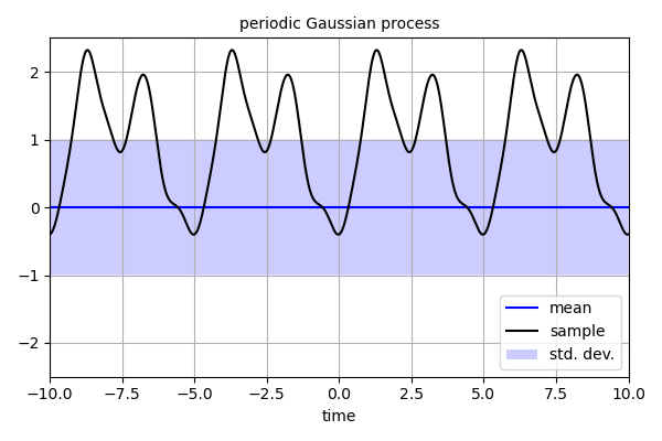
This script demonstrates how to create a periodic Gaussian process 
using the *gpiso* function.
'''
import numpy as np
import matplotlib.pyplot as plt
from sympy import sin, exp, pi 
from rbf.basis import get_r, get_eps, RBF
from rbf.gproc import gpiso
np.random.seed(1)

period = 5.0 
cls = 0.5 # characteristic length scale
var = 1.0 # variance

r = get_r() # get symbolic variables
eps = get_eps()
# create a symbolic expression of the periodic covariance function 
expr = exp(-sin(r*pi/period)**2/eps**2) 
# define a periodic RBF using the symbolic expression
basis = RBF(expr)
# define a Gaussian process using the periodic RBF
gp = gpiso(basis, eps=cls, var=var)
t = np.linspace(-10, 10, 1000)[:,None]
sample = gp.sample(t) # draw a sample
mu,sigma = gp(t) # evaluate mean and std. dev.

# plot the results
fig,ax = plt.subplots(figsize=(6,4))
ax.grid(True)
ax.plot(t[:,0], mu, 'b-', label='mean')
ax.fill_between(
    t[:,0], mu - sigma, mu + sigma,
    color='b', alpha=0.2, edgecolor='none', label='std. dev.')
ax.plot(t, sample, 'k', label='sample')
ax.set_xlim((-10.0, 10.0))
ax.set_ylim((-2.5*var, 2.5*var))
ax.legend(loc=4, fontsize=10)
ax.tick_params(labelsize=10)
ax.set_xlabel('time', fontsize=10)
ax.set_title('periodic Gaussian process', fontsize=10)
fig.tight_layout()
plt.savefig('../figures/gproc.e.png')
plt.show()

''' 
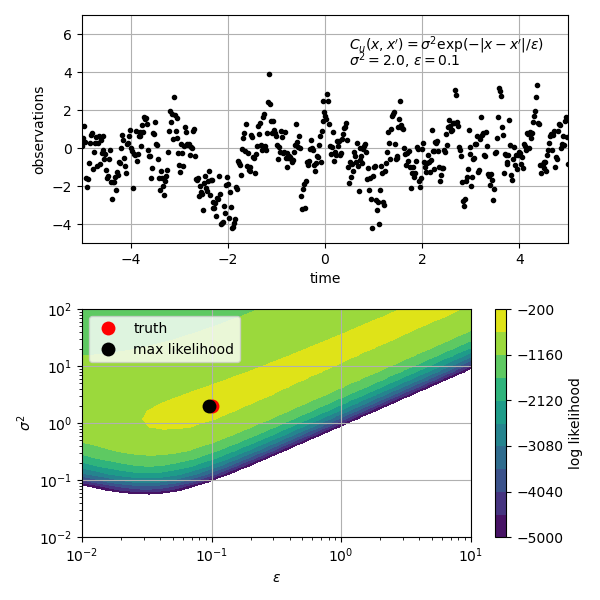
This script demonstrate how to optimize the hyperparameters for a 
Gaussian process based on the marginal likelihood. Optimization is 
performed in two ways, first with a grid search method and then with a 
downhill simplex method.
'''
import numpy as np
import matplotlib.pyplot as plt
from scipy.optimize import fmin
from rbf.gproc import gpiso
np.random.seed(3)

# True signal which we want to recover. This is a exponential function
# with mean=0.0, variance=2.0, and time-scale=0.1. For graphical
# purposes, we will only estimate the variance and time-scale.
eps = 0.1
var = 2.0
gp = gpiso('exp', eps=eps, var=var)

n = 500 # number of observations
time = np.linspace(-5.0, 5.0, n)[:,None] # observation points
data = gp.sample(time) # signal which we want to describe

# find the optimal hyperparameter with a brute force grid search
eps_search = 10**np.linspace(-2, 1, 30)
var_search = 10**np.linspace(-2, 2, 30)
log_likelihoods = np.zeros((30, 30))
for i, eps_test in enumerate(eps_search): 
  for j, var_test in enumerate(var_search): 
    gp = gpiso('exp', eps=eps_test, var=var_test)
    log_likelihoods[i, j] = gp.log_likelihood(time, data)

# find the optimal hyperparameters with a positively constrained 
# downhill simplex method
def fmin_pos(func, x0, *args, **kwargs):
  '''fmin with positivity constraint''' 
  def pos_func(x, *blargs):
    return func(np.exp(x), *blargs)

  out = fmin(pos_func, np.log(x0), *args, **kwargs)
  out = np.exp(out)
  return out

def objective(x, t, d):
  '''objective function to be minimized'''
  gp = gpiso('exp', eps=x[0], var=x[1])
  return -gp.log_likelihood(t,d)

# maximum likelihood estimate
eps_mle, var_mle = fmin_pos(objective, [1.0, 1.0], args=(time, data))

# plot the results
fig, axs = plt.subplots(2, 1, figsize=(6, 6))
ax = axs[0]
ax.grid(True)
ax.plot(time[:,0], data, 'k.', label='observations')
ax.set_xlim((-5.0, 5.0))
ax.set_ylim((-5.0, 7.0))
ax.set_xlabel('time', fontsize=10)
ax.set_ylabel('observations', fontsize=10)
ax.tick_params(labelsize=10)
ax.text(0.55, 0.85, r"$C_u(x,x') = \sigma^2\exp(-|x - x'|/\epsilon)$", transform=ax.transAxes)
ax.text(0.55, 0.775, r"$\sigma^2 = %s$, $\epsilon = %s$" % (var, eps), transform=ax.transAxes)
           
ax = axs[1]
ax.set_yscale('log')
ax.set_xscale('log')
ax.set_xlabel(r'$\epsilon$', fontsize=10)
ax.set_ylabel(r'$\sigma^2$', fontsize=10)
ax.tick_params(labelsize=10)
p = ax.contourf(eps_search, var_search, log_likelihoods.T, np.linspace(-5000.0, -200.0, 11), cmap='viridis')
cbar = plt.colorbar(p, ax=ax)
ax.plot([eps], [var], 'ro', markersize=10, mec='none', label='truth')
ax.plot([eps_mle], [var_mle], 'ko', markersize=10, mec='none', label='max likelihood')
ax.legend(fontsize=10, loc=2)
cbar.set_label('log likelihood', fontsize=10)
cbar.ax.tick_params(labelsize=10)
ax.grid(True)
plt.tight_layout()
plt.savefig('../figures/gproc.f.png')
plt.show()

''' 
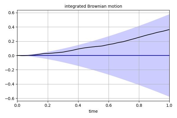
This script demonstrates how create a Gaussian process describing 
integrated Brownian motion with the *GaussianProcess* class. 
integrated Brownian motion has mean u(t) = 0 and covariance 

  cov(t1, t2) = (1/2)*min(t1, t2)**2 * (max(t1, t2) - min(t1, t2)/3).

It also demonstrates how to make the *GaussianProcess* differentiable 
by manually specifying the covariance derivatives.

'''
import numpy as np
import matplotlib.pyplot as plt
from rbf.gproc import GaussianProcess
np.random.seed(1)

# define mean function
def mean(x, diff):
  '''mean function which is zero for all derivatives'''
  out = np.zeros(x.shape[0])
  return out

# define covariance function
def cov(x1, x2, diff1, diff2):
  '''covariance function and its derivatives'''
  x1, x2 = np.meshgrid(x1[:, 0], x2[:, 0], indexing='ij')
  if (diff1 == (0,)) & (diff2 == (0,)):
    # integrated brownian motion
    out = (0.5*np.min([x1, x2], axis=0)**2*
           (np.max([x1, x2], axis=0) - 
            np.min([x1, x2], axis=0)/3.0))

  elif (diff1 == (1,)) & (diff2 == (1,)):
    # brownian motion
    out = np.min([x1, x2], axis=0)
  
  elif (diff1 == (1,)) & (diff2 == (0,)):   
    # derivative w.r.t x1
    out = np.zeros_like(x1)
    idx1 = x1 >= x2
    idx2 = x1 <  x2
    out[idx1] = 0.5*x2[idx1]**2
    out[idx2] = x1[idx2]*x2[idx2] - 0.5*x1[idx2]**2

  elif (diff1 == (0,)) & (diff2 == (1,)):   
    # derivative w.r.t x2
    out = np.zeros_like(x1)
    idx1 = x2 >= x1
    idx2 = x2 <  x1
    out[idx1] = 0.5*x1[idx1]**2
    out[idx2] = x2[idx2]*x1[idx2] - 0.5*x2[idx2]**2
  
  else:
    raise ValueError(
      'The *GaussianProcess* is not sufficiently differentiable')
  
  return out

t = np.linspace(0.0, 1, 100)[:, None]
gp = GaussianProcess(mean, cov, dim=1, differentiable=True)
sample = gp.sample(t) # draw a sample
mu, sigma = gp(t) # evaluate the mean and std. dev.

# plot the results
fig, ax = plt.subplots(figsize=(6, 4))
ax.grid(True)
ax.plot(t[:, 0], mu, 'b-', label='mean')
ax.fill_between(t[:, 0], mu+sigma, mu-sigma, color='b', alpha=0.2, edgecolor='none', label='std. dev.')
ax.plot(t[:, 0], sample, 'k', label='sample')
ax.set_xlabel('time', fontsize=10)
ax.set_xlim((0, 1))
ax.set_title('integrated Brownian motion', fontsize=10)
ax.tick_params(labelsize=10)
fig.tight_layout()
plt.savefig('../figures/gproc.g.png')
plt.show()