basis

This module contains the RBF class, which is used to symbolically define and numerically evaluate a radial basis function. RBF instances have been predefined in this module for some of the commonly used radial basis functions. The predefined radial basis functions are shown in the table below. For each expression in the table, \(r = ||x - c||_2\) and \(\epsilon\) is a shape parameter. \(x\) and \(c\) are the evaluation points and radial basis function centers, respectively.

The below table also shows the conditionally positive definite (CPD) order for each RBF. The definition of the CPD order can be found in Section 7.1. of [1]. For practical purposes, the CPD order is used to determine the degree of the polynomial that should accompany the RBF so that the interpolation problem or PDE being solved is well-posed. If solving an interpolation problem/PDE with an RBF that has CPD order m, then the functional form of the solution should include a polynomial with degree m-1. If the CPD order is 0, the RBF is positive definite and requires no additional polynomial.

Name	Expression	CPD Order
phs8 (8th-order polyharmonic spline)	\(-(\epsilon r)^8\log(\epsilon r)\)	5
phs7 (7th-order polyharmonic spline)	\((\epsilon r)^7\)	4
phs6 (6th-order polyharmonic spline)	\((\epsilon r)^6\log(\epsilon r)\)	4
phs5 (5th-order polyharmonic spline)	\(-(\epsilon r)^5\)	3
phs4 (4th-order polyharmonic spline)	\(-(\epsilon r)^4\log(\epsilon r)\)	3
phs3 (3rd-order polyharmonic spline)	\((\epsilon r)^3\)	2
phs2 (2nd-order polyharmonic spline)	\((\epsilon r)^2\log(\epsilon r)\)	2
phs1 (1st-order polyharmonic spline)	\(-\epsilon r\)	1
mq (multiquadric)	\(-(1 + (\epsilon r)^2)^{1/2}\)	1
imq (inverse multiquadric)	\((1 + (\epsilon r)^2)^{-1/2}\)	0
iq (inverse quadratic)	\((1 + (\epsilon r)^2)^{-1}\)	0
ga (Gaussian)	\(\exp(-(\epsilon r)^2)\)	0
exp (exponential)	\(\exp(-r/\epsilon)\)	0
se (squared exponential)	\(\exp(-r^2/(2\epsilon^2))\)	0
mat32 (Matern, v = 3/2)	\((1 + \sqrt{3} r/\epsilon)\exp(-\sqrt{3} r/\epsilon)\)	0
mat52 (Matern, v = 5/2)	\((1 + \sqrt{5} r/\epsilon + 5r^2/(3\epsilon^2))\exp(-\sqrt{5} r/\epsilon)\)	0
wen10 (Wendland, dim=1, k=0)	\((1 - r/\epsilon)_+\)	0
wen11 (Wendland, dim=1, k=1)	\((1 - r/\epsilon)_+^3(3r/\epsilon + 1)\)	0
wen12 (Wendland, dim=1, k=2)	\((1 - r/\epsilon)_+^5(8r^2/\epsilon^2 + 5r/\epsilon + 1)\)	0
wen30 (Wendland, dim=3, k=0)	\((1 - r/\epsilon)_+^2\)	0
wen31 (Wendland, dim=3, k=1)	\((1 - r/\epsilon)_+^4(4r/\epsilon + 1)\)	0
wen32 (Wendland, dim=3, k=2)	\((1 - r/\epsilon)_+^6(35r^2/\epsilon^2 + 18r/\epsilon + 3)/3\)	0

References

[1] Fasshauer, G., Meshfree Approximation Methods with Matlab. World Scientific Publishing Co, 2007.

class rbf.basis.RBF(*args, **kwargs)

Stores a symbolic expression of a Radial Basis Function (RBF) and evaluates the expression numerically when called.

Parameters:

• expr (sympy expression) – Sympy expression for the RBF. This must be a function of the symbolic variable r. r is the Euclidean distance to the RBF center. The expression may optionally be a function of the shape parameter eps. If eps is not provided then r is substituted with r*eps. The symbolic variables r and eps can be created with r, eps = sympy.symbols(‘r, eps’) or can be retrieved through the module-level attributes R and EPS.

• tol (float or sympy expression, optional) –

  Distance from the RBF center within which the RBF expression or its derivatives are not numerically stable. The symbolically evaluated limit at the center is returned when evaluating points where r <= tol. This can be a float or a sympy expression containing eps.

  If the limit of the RBF at its center is known, then it can be manually specified with the limits arguments.

• supp (float or sympy expression, optional) – The support for the RBF if it is compact. The RBF is set to zero where r > supp, regardless of what expr evaluates to. This can be a float or a sympy expression containing eps. This should be preferred over using a piecewise expression for compact RBFs due to difficulties sympy has with evaluating limits of piecewise expressions.

• limits (dict, optional) – Contains the values of the RBF or its derivatives at the center. For example, {(0,1): 2*eps} indicates that the derivative with respect to the second spatial dimension is 2*eps at x = c. If this dictionary is provided and tol is not None, then it will be searched before computing the limit symbolically.

• cpd_order (int, optional) – If the RBF is known to be conditionally positive definite, then specify the order here. This is saved as an attribute and is otherwise unused by this class.

Examples

Instantiate an inverse quadratic RBF

>>> from rbf.basis import *
>>> iq_expr = 1/(1 + (EPS*R)**2)
>>> iq = RBF(iq_expr)

Evaluate an inverse quadratic at 10 points ranging from -5 to 5. Note that the evaluation points and centers are two dimensional arrays

>>> x = np.linspace(-5.0, 5.0, 10)[:, None]
>>> center = np.array([[0.0]])
>>> values = iq(x, center)

Instantiate a sinc RBF. This has a singularity at the RBF center and it must be handled separately by specifying a number for tol.

>>> import sympy
>>> sinc_expr = sympy.sin(R)/R
>>> sinc = RBF(sinc_expr) # instantiate WITHOUT specifying `tol`
>>> x = np.array([[-1.0], [0.0], [1.0]])
>>> c = np.array([[0.0]])
>>> sinc(x, c) # this incorrectly evaluates to nan at the center
array([[ 0.84147098],
       [        nan],
       [ 0.84147098]])

>>> sinc = RBF(sinc_expr, tol=1e-10) # instantiate specifying `tol`
>>> sinc(x, c) # this now correctly evaluates to 1.0 at the center
array([[ 0.84147098],
       [ 1.        ],
       [ 0.84147098]])

__call__(x, c, eps=1.0, diff=None, out=None)

Numerically evaluates the RBF or its derivatives.

Parameters:

• x ((..., N, D) float array) – Evaluation points in D-dimensional space.

• c ((..., M, D) float array) – RBF centers in D-dimensional space.

• eps (float or float array, optional) – Shape parameter for each RBF.

• diff ((D,) int array, optional) – Derivative order for each dimension. For example, providing (2, 0, 1) would cause this function to return the RBF after differentiating it twice along the first dimension and once along the third dimension.

• out ((..., N, M) float array, optional) – Array in which the output is written.

Returns:

(…, N, M) float array – The RBFs with centers c evaluated at x.

Notes

When there are 15 or fewer spatial dimensions D, symbolic RBF expressions are converted to numeric functions with sympy’s ufuncify method. If there are more than 15 dimensions, the lambdify method is automatically used instead. However, functions produced by this method are unable to perform in-place operations. Hence, if both D > 15 and out are specified, in-place operations are emulated for compatibility. This preserves syntactic consistency with code in 15 dimensions or less, but incurs memory and performance overhead costs due to the creation of intermediate arrays.

The derivative order can be arbitrarily high, but some RBFs, such as Wendland and Matern, become numerically unstable when the derivative order exceeds 2.

center_value(eps=1.0, diff=(0,))

Returns the value at the center of the RBF for the given eps and diff. This is a faster alternative to determining the center value with __call__.

Parameters:

• eps (float, optional) – Shape parameter.

• diff (tuple, optional) – Derivative order for each dimension.

Returns:

float

clear_cache()

Clears the cache of numeric functions. Makes a cache dictionary if it does not already exist.

property eps_is_divisor

True if eps divides r in the RBF expression.

property eps_is_factor

True if eps multiplies r in the RBF expression.

class rbf.basis.SparseRBF(*args, **kwargs)

Stores a symbolic expression of a compact Radial Basis Function (RBF) and evaluates the expression numerically when called. Calling a SparseRBF instance will return a csc sparse matrix.

Parameters:

• expr (sympy expression) – Sympy expression for the RBF. This must be a function of the symbolic variable r. r is the Euclidean distance to the RBF center. The expression may optionally be a function of the shape parameter eps. If eps is not provided then r is substituted with r*eps. The symbolic variables r and eps can be created with r, eps = sympy.symbols(‘r, eps’) or can be retrieved through the module-level attributes R and EPS.

• supp (float or sympy expression) – The support for the RBF. The RBF is set to zero where r > supp, regardless of what expr evaluates to. This can be a float or a sympy expression containing eps.

• tol (float or sympy expression, optional) –

  Distance from the RBF center within which the RBF expression or its derivatives are not numerically stable. The symbolically evaluated limit at the center is returned when evaluating points where r <= tol. This can be a float or a sympy expression containing eps.

  If the limit of the RBF at its center is known, then it can be manually specified with the limits arguments.

• limits (dict, optional) – Contains the values of the RBF or its derivatives at the center. For example, {(0,1): 2*eps} indicates that the derivative with respect to the second spatial dimension is 2*eps at x = c. If this dictionary is provided and tol is not None, then it will be searched before computing the limit symbolically.

• cpd_order (int, optional) – If the RBF is known to be conditionally positive definite, then specify the order here. This is saved as an attribute and is otherwise unused by this class.

__call__(x, c, eps=1.0, diff=None)

Numerically evaluates the RBF or its derivatives.

Parameters:

• x ((N, D) float array) – Evaluation points in D-dimensional space.

• c ((M, D) float array) – RBF centers in D-dimensional space.

• eps (float, optional) – Shape parameter.

• diff ((D,) int array, optional) – Derivative order for each dimension. For example, providing (2, 0, 1) would cause this function to return the RBF after differentiating it twice along the first dimension and once along the third dimension.

Returns:

out ((N, M) csc sparse matrix) – The RBFs with centers c evaluated at x.

rbf.basis.get_rbf(value)

Returns the RBF corresponding to value. If value is a string, then this return the correspondingly named predefined RBF. If value is an RBF instance then this returns value.

Examples

''' 
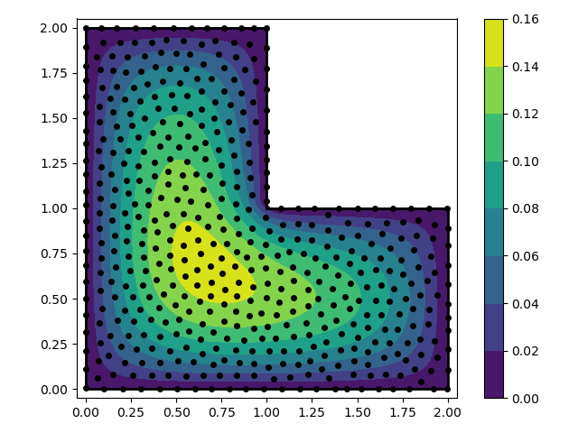
In this example we solve the Poisson equation over an L-shaped domain with
fixed boundary conditions. We use the multiquadratic RBF (`mq`)
'''
import numpy as np
from rbf.basis import mq
from rbf.pde.geometry import contains
from rbf.pde.nodes import poisson_disc_nodes
import matplotlib.pyplot as plt

# Define the problem domain with line segments.
vert = np.array([[0.0, 0.0], [2.0, 0.0], [2.0, 1.0],
                 [1.0, 1.0], [1.0, 2.0], [0.0, 2.0]])
smp = np.array([[0, 1], [1, 2], [2, 3], [3, 4], [4, 5], [5, 0]])

spacing = 0.07 # approximate spacing between nodes

eps = 0.3/spacing  # shape parameter

# generate the nodes. `nodes` is a (N, 2) float array, `groups` is a dict
# identifying which group each node is in
nodes, groups, _ = poisson_disc_nodes(spacing, (vert, smp)) 
N = nodes.shape[0]

# create "left hand side" matrix
A = np.empty((N, N))
A[groups['interior']] = mq(nodes[groups['interior']], nodes, eps=eps, diff=[2, 0])
A[groups['interior']] += mq(nodes[groups['interior']], nodes, eps=eps, diff=[0, 2])
A[groups['boundary:all']] = mq(nodes[groups['boundary:all']], nodes, eps=eps)

# create "right hand side" vector
d = np.empty(N)
d[groups['interior']] = -1.0 # forcing term
d[groups['boundary:all']] = 0.0 # boundary condition

# Solve for the RBF coefficients
coeff = np.linalg.solve(A, d) 

# interpolate the solution on a grid
xg, yg = np.meshgrid(np.linspace(0.0, 2.02, 100),
                     np.linspace(0.0, 2.02, 100))
points = np.array([xg.flatten(), yg.flatten()]).T                    
u = mq(points, nodes, eps=eps).dot(coeff)
# mask points outside of the domain
u[~contains(points, vert, smp)] = np.nan 
# fold the solution into a grid
ug = u.reshape((100, 100))
# make a contour plot of the solution
fig, ax = plt.subplots()
p = ax.contourf(xg, yg, ug, np.linspace(0.0, 0.16, 9), cmap='viridis')
ax.plot(nodes[:, 0], nodes[:, 1], 'ko', markersize=4)
for s in smp:
  ax.plot(vert[s, 0], vert[s, 1], 'k-', lw=2)

ax.set_aspect('equal')
ax.set_xlim(-0.05, 2.05)
ax.set_ylim(-0.05, 2.05)
fig.colorbar(p, ax=ax)
fig.tight_layout()
plt.savefig('../figures/basis.a.png')
plt.show()

''' 
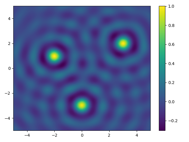
In this script we define and plot an RBF which is based on the sinc 
function
'''
import numpy as np
import sympy
import matplotlib.pyplot as plt
from rbf.basis import RBF, get_r, get_eps

r, eps = get_r(), get_eps() # get symbolic variables
expr = sympy.sin(eps*r)/(eps*r) # symbolic expression for the RBF
sinc_rbf = RBF(expr) # instantiate the RBF
x = np.linspace(-5, 5, 500)
points = np.reshape(np.meshgrid(x, x), (2, 500*500)).T # interp points
centers = np.array([[0.0, -3.0], [3.0, 2.0], [-2.0, 1.0]]) # RBF centers
eps = np.array([5.0, 5.0, 5.0]) # shape parameters
values = sinc_rbf(points, centers, eps=eps) # Evaluate the RBFs

# plot the sum of each RBF
fig, ax = plt.subplots()
p = ax.tripcolor(points[:, 0], points[:, 1], np.sum(values, axis=1),
                 shading='gouraud', cmap='viridis')
plt.colorbar(p, ax=ax)
ax.set_xlim((-5, 5))
ax.set_ylim((-5, 5))
plt.tight_layout()
plt.savefig('../figures/basis.b.png')
plt.show()